1

“Fault Detection

in Wireless Sensor Network Using

Distributed Approach”

A Thesis submitted in partial fulfillment of the requirements for the degree of

Bachelor of Technology

in

Computer Science & Engineering

by

Amlan Kumar Nayak Bibhas MishraRoll No: 108CS026 Roll No: 108CS020

Department of Computer Science & Engineering

National Institute of Technology Rourkela

Rourkela, Orissa, 769 008, India

May 2012

2

Department of Computer Science & Engineering

National Institute of Technology

Rourkela, 769008

CERTIFICATE

This is to certify that the thesis entitled, “Distributed Fault Detection In Wireless Sensor

Networks” by Mr. Amlan Kumar Nayak & Mr. Bibhas Mishra in partial fulfillment of the

requirements for the award of Bachelor of Technology Degree in Computer Science &

Engineering at the National Institute of Technology, Rourkela is an authentic work carried out by

them under my supervision and guidance.

To the best of my knowledge the matter embodied in the thesis has not been submitted to any

other University/ Institute for the award of any Degree or Diploma.

Date: Prof. M.N Sahoo

Dept. of Computer Science & Engineering

National Institute of Technology

Rourkela-769008

3

ACKNOWLEDGEMENT

We would like to express our heartfelt thanks and gratitude to Professor M.N. Sahoo,

Department of Computer Science Engineering, NIT Rourkela, our guide and our mentor, who

was with us during every stage of the work; and whose guidance and valuable suggestions has

made this work possible.

Further, we would also like to thank all the faculty members and staff of Department of

Computer Science Engineering, NIT Rourkela for their invaluable support and help during the

entire project work.

We would love to thank our family members for encouraging us at every stage of this project

work. Last but not least, our sincere thanks to all our friends who have patiently extended all

sorts of help for accomplishing this undertaking.

SUBMITTED BY:

Amlan Kumar Nayak BibhasMishra108CS026 108CS020

Computer Science & Engineering

National Institute of Technology Rourkela

4

ABSTRACT

In recent days, Wireless Sensor Networks are emerging as a promising and interesting area. Wireless Sensor Network consists of a large number of heterogeneous/homogeneous sensor nodes which communicates through wireless medium and works cooperatively to sense or monitor the environment. The number of sensor nodes in a network can vary from hundreds to thousands. The node senses data from environment and sends these data to the gateway node. Mostly WSNs are used for applications such as military surveillance and disaster monitoring. We propose a distributed localized faulty sensor detection algorithm where each sensor identifies its own status to be either ”good” or ”faulty” which is then supported by its neighbors as they also check the node behavior. Finally, the algorithm is tested under different number of faulty sensors in the same area. Our Simulation results demonstrate that the time consumed to find out the faulty nodes in our proposed algorithm is relatively less with a large number of faulty sensors existing in the network.

5

Contents1. INTRODUCTION .................................................................................................................................. 9

1.1 What is WSN?................................................................................................................................... 9

1.2 Introduction to WSN ......................................................................................................................... 9

1.3 WSN application ............................................................................................................................. 10

1.4 Sensor Network application classes ................................................................................................ 11

1.4.1 Environmental data collection................................................................................................. 11

1.4.2 Security Monitoring ................................................................................................................ 12

1.4.3 Node tracking scenarios .......................................................................................................... 12

1.5 WSN System Architecture ............................................................................................................. 13

1.5.1 Networking Topologies............................................................................................................ 13

2. LITERATURE REVIEW ..................................................................................................................... 16

2.1 A Self-Managing Fault Management Mechanism for WSN........................................................... 16

2.1.1 Fault Detection and Diagnosis ................................................................................................ 16

2.1.2 Fault Recovery ........................................................................................................................ 18

2.2 Distributed Fault Detection in WSN ............................................................................................... 20

2.2.1 Definition ................................................................................................................................. 20

2.2.3 An Example ............................................................................................................................. 23

3 PROPOSED MECHANISM................................................................................................................. 27

3.1 Network model and Fault model.................................................................................................... 27

3.3 Issues in the Existing Algorithm ..................................................................................................... 28

3.4 Proposed Algorithm ........................................................................................................................ 29

4. SIMULATION AND RESULTS......................................................................................................... 32

4.1 Existing Algorithm......................................................................................................................... 32

4.2 Improved Algorithm ...................................................................................................................... 34

5. CONCLUSION ...................................................................................................................................... 38

5.1 Conclusion ...................................................................................................................................... 38

5.2 Future work ..................................................................................................................................... 38

REFERENCES 39

6

LIST OF FIGURES

Figure 1.1 WSN Application Areas…………………………………………. …... 11

Figure 1.2 WSN Network Topologies………………………………………. .….. 14

Figure 2.1 Fault Detection and Diagnosis Process……………………………….. 17

Figure 2.2 Virtual Grid of Nodes…………………………………………………. 18

Figure 2.3 A partial set of sensor nodes in a WSN with faulty sensors…………... 23

Figure 3.1.Sensor nodes randomly deployed over an area……………………….. 27

Figure 4.1. Comparison of No. of Nodes Vs Time Elapsed……………………… 36

7

LIST OF TABLES

Table 2.1 Analysis of Faults………………………………………………………. 25

8

CHAPTER 1

INTRODUCTION

9

1. INTRODUCTION

1.1 What is WSN?Wireless sensor networks have seen tremendous advances and utilization in the past two decades. Starting from petroleum exploration, mining, weather and even battle operations, all of these require sensor applications. One reason behind the growing popularity of wireless sensors is that they can work in remote areas without manual intervention. All the user needs to do is to gather the data sent by the sensors, and with certain analysis extract meaningful information from them. Usually sensor applications involve many sensors deployed together. These sensors form a network and collaborate with each other to gather data and send it to the base station. The base station acts as the control centre where the data from the sensors are gathered for further analysis and processing. In a nutshell, a wireless sensor network (WSN) is a wireless network consisting of spatially distributed nodes which use sensors to monitor physical or environmental conditions. These nodes combine with routers and gateways to create a WSN system.

1.2 Introduction to WSNThe WSN is made of nodes from a few to several hundred, where each node is connected to one or several sensors.The basic components of a node are

o Sensor and actuator - an interface to the physical world designed to sense the environmental parameters like pressure and temperature.

o Controller - is to control different modes of operation for processing of datao Memory - storage for programming data.o Communication - a device like antenna for sending and receiving data over a wireless

channel.o Power Supply- supply of energy for smooth operation of a node like battery.

The topology of the WSNs can vary from a simple star network to an advanced wireless mesh network. The propagation technique among the nodes of the network could be routing or flooding. The power of the wireless sensor networks lies in the capability to deploy large numbers of small nodes that assemble and configure themselves. In addition to drastically decreasing the installation costs, wireless sensor networks have the capability to dynamically adapt to changing environments. Adaptation mechanisms can lead to changes in network topologies or can cause the network to shift between different modes of operation.

The characteristics of sensor nodes are as follows:o Resource Constrainto Unknown topology before deploymento Unattended and unprotected once deployed

o Unreliable wireless communication

10

Due to the above characteristics, WSN are easily vulnerable to attacks. Providing security solutions to these networks is difficult due to its characteristics such as tiny nature and constraints in resources.

1.3 WSN application

? Area Monitoring: It is a common application of WSNs. Here the WSN is deployed over a region where some event is to be monitored. A military example is the use of sensors to diagnosis enemy intrusion [6]. When the sensors detect the event being monitored, the event is reported to one of the base stations, which then takes relevant action. Similarly, wireless sensor networks may use a range of sensors to detect the presence/absence of vehicles ranging from motorcycles to train cars.

? Environmental Monitoring: Wireless sensor networks have been deployed in several cities to monitor the concentration of dangerous gases for citizens. Wireless sensor networks can also be used to reduce the temperature and humidity levels inside greenhouses [6].

? Medical Application: Sensor networks may also be broadly used in health care centres. In some modern hospital sensor networks are designed to supervise patient physiological data, to reduce the drug administration track and monitor patients and doctors inside the hospital.

? Structural monitoring: Wireless sensors are used to monitor the movement within large buildings and infrastructure such as bridges, flyovers, embankments, tunnels etc.

? Traffic Monitoring: The sensor node has a built-in magneto-resistive sensor that measures changes in the Earth's magnetic field caused by the existence or passing of a vehicle in the proximity of the node [7]. By placing two nodes a few metres apart in the direction of traffic, accurate individual vehicle speeds can be calculated and reported.

? Habitat Monitoring: The intimate connection with its immediate physical environment allows each sensor to provide localized measurements and detailed report which is hard to obtain through traditional instrumentation.

11

Remote Monitoring sustainability Industrial Measurements

Air/Climate Water/Soil Indoor Monitoring Power system Solar Wind Farm

12

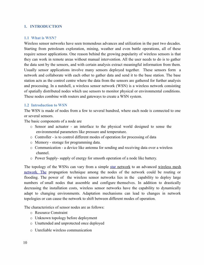
Structural Monitoring Machine Monitoring Process Monitoring

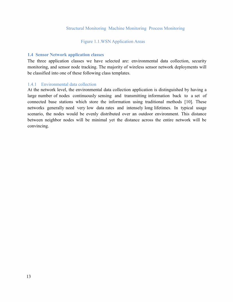
Figure 1.1.WSN Application Areas

1.4 Sensor Network application classesThe three application classes we have selected are: environmental data collection, security monitoring, and sensor node tracking. The majority of wireless sensor network deployments will be classified into one of these following class templates.

1.4.1 Environmental data collectionAt the network level, the environmental data collection application is distinguished by having a large number of nodes continuously sensing and transmitting information back to a set of connected base stations which store the information using traditional methods [10]. These networks generally need very low data rates and intensely long lifetimes. In typical usage scenario, the nodes would be evenly distributed over an outdoor environment. This distance between neighbor nodes will be minimal yet the distance across the entire network will be convincing.

13

After deployment, the nodes must first discover the topology of the network and evaluate optimal routing strategies. The routing strategy may then be used to route the data to a central collection points. In environmental monitoring applications, it is not essential that the nodes establish the optimal routing strategies on their own. Instead, it may be possible to compute the optimal routing topology outside of the network and then communicate the necessary information to the nodes as required which is possible because the physical topology of the network is relatively constant [11].

1.4.2 Security MonitoringOur second class of sensor network application is security monitoring. Security monitoring networks are built of nodes which are placed at fixed locations throughout an environment that continuously control one or more sensors to detect an anomaly. A major difference between security monitoring and environmental monitoring is that security networks do not collect any data. This leads to a significant impact on the optimal network architecture .Each node frequently check the status of its sensors but it only transmit a data report when there will a security violation. The immediate and reliable communication among the alarm messages is the system’s primary requirement. These are the report generated by exception networks.

Additionally, it is essential that it is validated that each node is still present and working. If a node is disabled or fail, it will represent a security violation that must be reported. For security monitoring applications, the network should be configured so that nodes are responsible for finding the status of each other. We have one approach where each node is assigned to peer that will report if a node does not function. The optimal topology of a security monitoring network will look quite different from that of a data collection network.

Once detected, a security violation should be communicated to the connected station immediately. The latency of the information communication across the network to the base station has a severe impact on application performance. Users demand that alarm situations should be reported within seconds of detection. This means that network nodes should be able to respond readily to requests from their neighbors to forward data [13].

1.4.3 Node tracking scenariosA third usage scenario commonly analyzed for wireless sensor networks is the tracing of a tagged object through a region of space controlled by a sensor network. There are various situations where one would like to trace the location of valuable assets or personnel. Current control systems attempt to track objects by recording the last checkpoint which an object passed through. However, with these traditional systems it is not easily possible to determine the object’s current location. For example, UPS tracks every shipment by scanning it with a barcode whenever it passes through a routing center. The system breaks down when objects do not flow from checkpoint to checkpoint. In typical work environments it is not practical to expect objects to be continuously passed through checkpoints.

14

Using wireless sensor networks, objects can be traced by simply tagging them with a tiny sensor node. The sensor node will be traced as it moves through an area of sensor nodes which are deployed in the environment at known locations. Instead of sensing the environmental data, these nodes will be deployed to sense the messages of the nodes which are attached to various objects. The nodes may be used as active tags which announce the presence of a device. A database may be used to record the location of traced objects relative to the large set of nodes at known locations.

1.5 WSN System ArchitectureIn a common Wireless Sensor Network architecture, the measurement nodes are deployed to calculate measurements such as temperature, voltage, heat, or even dissolved oxygen. The nodes are part of a wireless sensor network administered by the gateway that governs network aspects such as client authentication and data security [14]. The gateway collects the measurement data from each and every node and sends it through a wired connection, typically Ethernet, to a host controller.

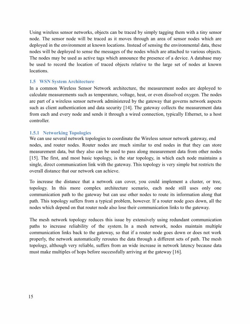
1.5.1 Networking TopologiesWe can use several network topologies to coordinate the Wireless sensor network gateway, endnodes, and router nodes. Router nodes are much similar to end nodes in that they can store measurement data, but they also can be used to pass along measurement data from other nodes [15]. The first, and most basic topology, is the star topology, in which each node maintains a single, direct communication link with the gateway. This topology is very simple but restricts the overall distance that our network can achieve.

To increase the distance that a network can cover, you could implement a cluster, or tree, topology. In this more complex architecture scenario, each node still uses only one communication path to the gateway but can use other nodes to route its information along that path. This topology suffers from a typical problem, however. If a router node goes down, all the nodes which depend on that router node also lose their communication links to the gateway.

The mesh network topology reduces this issue by extensively using redundant communication paths to increase reliability of the system. In a mesh network, nodes maintain multiple communication links back to the gateway, so that if a router node goes down or does not work properly, the network automatically reroutes the data through a different sets of path. The mesh topology, although very reliable, suffers from an wide increase in network latency because data must make multiples of hops before successfully arriving at the gateway [16].

15

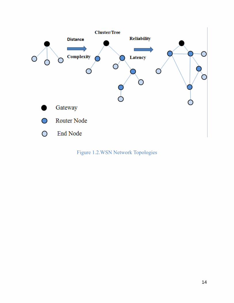
Figure 1.2.WSN Network Topologies

14

CHAPTER 2

LITERATURE REVIEW

17

2. LITERATURE REVIEW

In this section, we like to give a brief review of the different schemes that we have studied for

wireless sensor networks.

2.1 A Self-Managing Fault Management Mechanism for WSN

In this approach a new fault management mechanism was proposed to deal with fault detection and recovery. It proposes a hierarchical structure to properly distribute fault management tasks among sensor nodes by heavily introducing more self-managing functions. The proposed failure detection and recovery algorithms have been compared with some existing related algorithm and proven to be more energy efficient.

The proposed fault management mechanism can be divided into two phases:o Fault detection and diagnosiso Fault recovery

2.1.1 Fault Detection and DiagnosisDetection of faulty sensor nodes can be achieved by two mechanisms i.e. self-detection (or passive-detection) and active-detection. In self-detection, sensor nodes are required to periodically monitor their residual energy, and identify the potential failure. In this scheme, we consider the battery depletion as a main cause of node sudden death. A node is termed as failing when its energy drops below the threshold value. When a common node is failing due to energy depletion, it sends a message to its cell manager that it is going to sleep mode due to energy below the threshold value [17]. This requires no recovery steps. Self-detection is considered as a local computational process of sensor nodes, and requires less in-network communication to conserve the node energy. In addition, it also reduces the response delay of the management system towards the potential failure of sensor nodes [18].

To efficiently detect the node sudden death, our fault management system employed an active detection mode. In this approach, the message of updating the node residual battery is applied to track the existence of sensor nodes. In active detection, cell manager asks its cell members on regular basis to send their updates. Such as the cell manager sends “get” messages to the associated common nodes on regular basis and in return nodes send their updates. This is called in-cell update cycle. The update_msg consists of node ID, energy and location information. As shown in figure 2.1, exchange of update messages takes place between cell manager and its cell members. If the cell manager does not receive an update from any node then it sends an instant message to the node acquiring about its status [19]. If cell manager does not receive the acknowledgement in a given time, it then declares the node faulty and passes this information to the remaining nodes in the cell. Cell managers only concentrate on its cell members and only inform the group manager for further assistant if the network performance of its small region has been in a critical level.

18

Figure 2.1.Fault Detection and Diagnosis Process

A cell manager also employs the self-detection approach and regularly monitors its residual energy status. All sensor nodes start with the same residual energy. After going through various transmissions, the node energy decreases. If the node energy becomes less than or equal to 20% of battery life, the node is ranked as low energy node and becomes liable to put to sleep. If the node energy is greater or equal to 50% of the battery life, it is ranked as high and becomes the promising candidate for the cell manager. Thus, if a cell manager residual energy becomes less than or equal to 20% of battery life, it then triggers the alarm and notifies its cell members and the group manager of its low energy status and appoints a new cell manager to replace it.

Every cell manager sends health status information to its group manager. This is called out-cell update cycle and are less frequent than in-cell update cycle. If a group manager does not hear from a particular cell manager during out-cell update cycle, it then sends a quick reminder to the cell manager and enquires about its status. If the group manager does not hear from the same cell manager again during second update cycle, it then declares the cell manager faulty and informs its cell members [20]. This approach is used to detect the sudden death of a cell manager. Group manager also monitor its health status regularly and respond when its residual energy drops below the threshold value. It notifies its cell members and neighboring group managers of its low energy status and an indication to appoint a new group manager. Sudden death of a group manager can be detected by the base station. If the bases station does not receive any traffic from a particular group manager, it then consults the group manager and asks for its current status. If the base station does not receive any acknowledgement, it then considers the group manager faulty (sudden death) and propagates this information to its cell managers. The base station

19

primarily focuses on the existence of the group managers from their sudden death. Meanwhile, the group managers and cell managers take most parts in passive and active detection in the network.

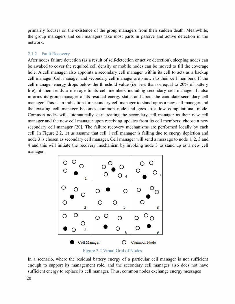
2.1.2 Fault RecoveryAfter nodes failure detection (as a result of self-detection or active detection), sleeping nodes can be awaked to cover the required cell density or mobile nodes can be moved to fill the coverage hole. A cell manager also appoints a secondary cell manager within its cell to acts as a backup cell manager. Cell manager and secondary cell manager are known to their cell members. If the cell manager energy drops below the threshold value (i.e. less than or equal to 20% of battery life), it then sends a message to its cell members including secondary cell manager. It also informs its group manager of its residual energy status and about the candidate secondary cell manager. This is an indication for secondary cell manager to stand up as a new cell manager and the existing cell manager becomes common node and goes to a low computational mode. Common nodes will automatically start treating the secondary cell manager as their new cell manager and the new cell manager upon receiving updates from its cell members; choose a new secondary cell manager [20]. The failure recovery mechanisms are performed locally by each cell. In Figure 2.2, let us assume that cell 1 cell manager is failing due to energy depletion and node 3 is chosen as secondary cell manager. Cell manager will send a message to node 1, 2, 3 and 4 and this will initiate the recovery mechanism by invoking node 3 to stand up as a new cell manager.

Figure 2.2.Virual Grid of Nodes

In a scenario, where the residual battery energy of a particular cell manager is not sufficient enough to support its management role, and the secondary cell manager also does not have sufficient energy to replace its cell manager. Thus, common nodes exchange energy messages

20

within the cell to appoint a new cell manager with residual energy greater or equal to 50% of battery life. In addition, if there is no candidate node within the cell that has sufficient energy to replace the cell manager. The event cell manager sends a request to its group manager to merge the remaining nodes with the neighboring cells.

When a group manager detects the sudden death of a cell manager, it then informs the cell members of that faulty cell manager (including the secondary cell manager). This is an indication for the secondary cell manager to start acting as a new cell manager. A group manager also maintains a backup node within the group to replace it when required. If the group manager residual energy drops below the threshold value (i.e. greater or equal to 50% of battery life), it may downgrade itself to a common node or enter into a sleep mode, and notify its backup node to replace it. The information of this change is propagated to neighboring group managers and cell managers within the group. As a result of group manager sudden death, the backup node will receive a message from the base station to start acting as the new group manager. If the backup node does not have enough energy to replace the group manager, cell managers within a group co-ordinate to appoint a new group manager for themselves based on residual energy.

Each cell maintains its health status in terms of energy. It can be High, Medium or Low. These health statuses are then sent out to their associate group managers periodically during out- cell update cycle. Upon receiving these health statuses, group manager predict and avoid future faults. For example; if a cell has health status high then group manager always recommends that cell for any operation or routing but if the health status is medium then group manager will occasionally recommend it for any operation [21]. Health status Low means that the cell has insufficient energy and should be avoided for any operation. Therefore, a group manager can easily avoid using cells with low health status or alternatively, instruct the low health status cell to join the neighboring cell.

Consider Figure 2.2, let cell 4 manager is a group manager and it receives health status updates from cell 1, 2 and 3. Cell 2 sends a health status low to its group manager, which alert group manager about the energy status of cell 2 [22].

21

2.2 Distributed Fault Detection in WSN

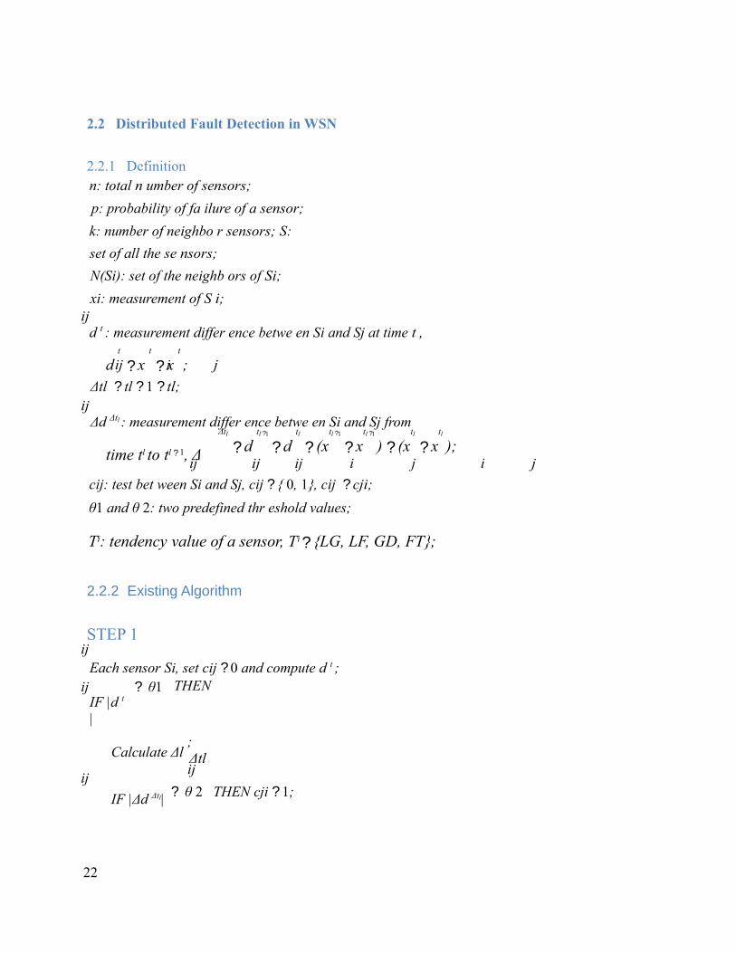
2.2.1 Definitionn: total n umber of sensors;

p: probability of fa ilure of a sensor;

k: number of neighbo r sensors; S:

set of all the se nsors;

N(Si): set of the neighb ors of Si;

xi: measurement of S i;ij

d t : measurement differ ence betwe en Si and Sj at time t ,

d t

? x t

? x t

;ij i j

Δtl ? tl ? 1 ? tl;ij

Δd Δtl : measurement differ ence betwe en Si and Sj from

time tl to tl ? 1, Δ

Δtl

? d tl ?1

? d tl

? (xtl ?1

? xtl ?1

) ? (xtl

? xtl

);ij ij ij i j i j

cij: test bet ween Si and Sj, cij ? { 0, 1}, cij ? cji;

θ1 and θ 2: two predefined thr eshold values;

Ti: tendency value of a sensor, Ti ? {LG, LF, GD, FT};

2.2.2 Existing Algorithm

STEP 1ij

Each sensor Si, set cij ? 0 and compute d t ;ij

IF |d t

|

? θ1 THEN

Calculate Δl;Δtlij

ij

IF |Δd Δtl| ? θ 2 THEN cji ? 1;

22

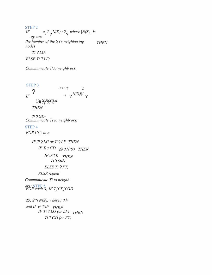
STEP 2IF

?Sj ? N(Si)

cij ?

?|N(Si)|/ 2?

, where |N(Si)| is

the number of the S i's neighboring nodes

Ti ? LG;

ELSE Ti ? LF;

Communicate Ti to neighb ors;

THEN

STEP 3

?1 ? 2 ij ? 2

IF ( Sj ? N(Si) a n d Tj ? LG

THEN

Ti ? GD;

c ) ?|N(Si)|/ ?

Communicate Ti to neighb ors;

STEP 4FOR i ? 1 to n

IF Ti ? LG or Ti ? LF THEN

IF Tj ? GD ?Sj ? N(Si) THEN

IF cij ? 0 THENTi ? GD;

ELSE Ti ? FT;

ELSE repeat

Communicate Ti to neighb

ors; STEP 5FOR each Si, IF Tj

? Th ? GD

?Sj, Sh ? N(Si), where j ? h,

and IF cji ? chi THEN

IF Ti ? LG (or LF)

Ti ? GD (or FT)THEN

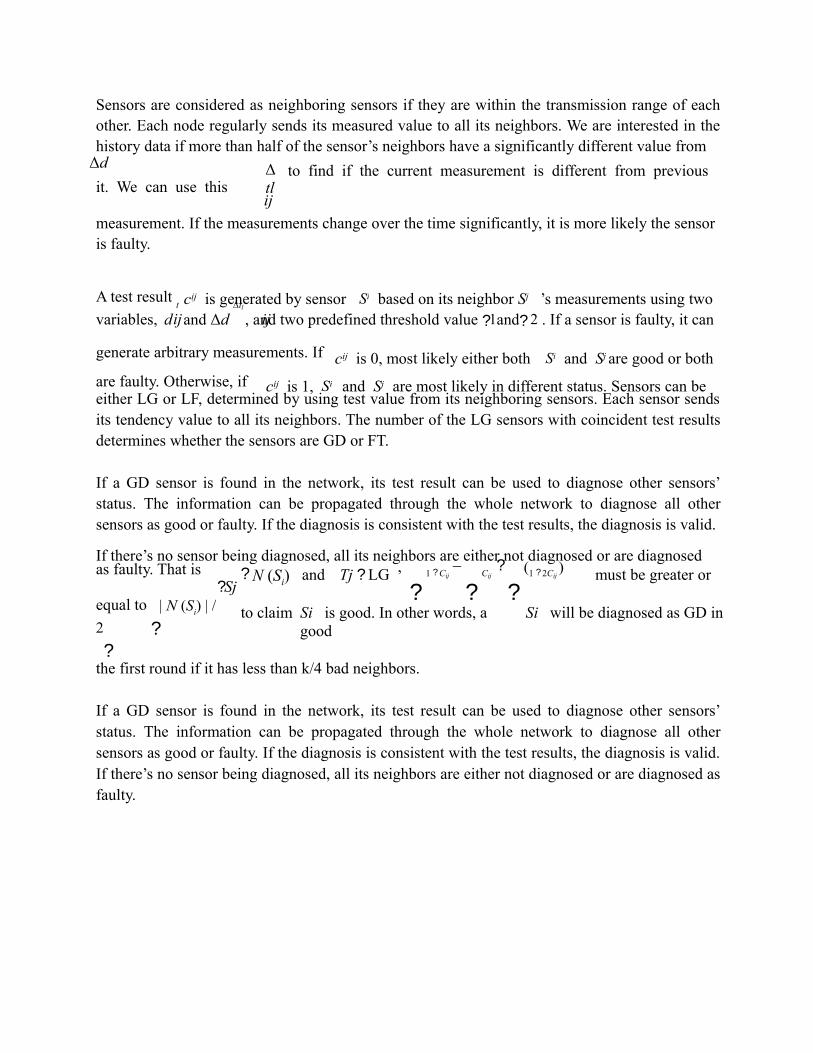
Sensors are considered as neighboring sensors if they are within the transmission range of each other. Each node regularly sends its measured value to all its neighbors. We are interested in the history data if more than half of the sensor’s neighbors have a significantly different value from

Δd

it. We can use thisΔtlij

to find if the current measurement is different from previous

measurement. If the measurements change over the time significantly, it is more likely the sensor is faulty.

A test result cij is generated by sensor Si based on its neighbor Sj ’s measurements using twovariables, d

t

and Δd Δtl

, and two predefined threshold value ?1and? 2 . If a sensor is faulty, it canij ij

generate arbitrary measurements. If cij is 0, most likely either both Si and Sj are good or both

are faulty. Otherwise, if cij is 1, Si and Sj are most likely in different status. Sensors can beeither LG or LF, determined by using test value from its neighboring sensors. Each sensor sends its tendency value to all its neighbors. The number of the LG sensors with coincident test results determines whether the sensors are GD or FT.

If a GD sensor is found in the network, its test result can be used to diagnose other sensors’ status. The information can be propagated through the whole network to diagnose all other sensors as good or faulty. If the diagnosis is consistent with the test results, the diagnosis is valid.

If there’s no sensor being diagnosed, all its neighbors are either not diagnosed or are diagnosedas faulty. That is

?Sj ? N (Si) and Tj ? LG ,

? 1 ? Cij

−

? Cij

?

? (1 ? 2Cij

) must be greater or

equal to

?| N (Si) | /

2

?

to claim Si is good. In other words, a good

Si will be diagnosed as GD in

the first round if it has less than k/4 bad neighbors.

If a GD sensor is found in the network, its test result can be used to diagnose other sensors’ status. The information can be propagated through the whole network to diagnose all other sensors as good or faulty. If the diagnosis is consistent with the test results, the diagnosis is valid. If there’s no sensor being diagnosed, all its neighbors are either not diagnosed or are diagnosed as faulty.

2.2.3 An Example

Figure 2.3.A partial set of sensor nodes in a WSN with faulty sensors

In this section, we present an example to illustrate our algorithm. Fig.2.3 shows a partial set of

sensor nodes in a wireless sensor network with some faulty nodes. NodesS1 − S 9 inside the

circle area are the nodes which we are interested in. If the two nodes are neighbors, they are

connected by dotted line. Communication between nodes outside the circle is not shown in the

figure. Each node inside the interested area is tested by its neighbors. Test results are either 0 or

1 depending upon the measurement difference and threshold value ? . Tendency value Ti is

finalized at the third iteration. Table 2.1 lists the analysis results obtained by applying the

Localized Fault Detection Algorithm. Four out of nine sensor nodes in the area are faulty. The

other five nodes are good and there is no ambiguity occurring in this example. Each node’s

neighbors with GD tendency value generate the same testing results when they determine the

node’s status.

First, each ofS1 − S 9 generates cij test results for all their neighbors in the way as specified in

step 1 of our algorithm. The results are shown under the 2nd and the 3rd columns of Table 2.1.

Secondly, S1 − S 9 decide their own tendency value, T 1 ? T 9 . If the summation of test results isless than half of the number of its

neighbors, the sensor is likely good.

Otherwise, it is likely faulty.

For example, for S1 ,

?Sj ? N ( S 1)

c1 j ? 1 ? ?| N (S1) | /2?

? 3

?? T 1 ? LG . The same test is

done for all

other nodes. For

S 2

?Sj ? N ( S 2 )

c2 j ? 3 ? ?| N (S 2) | /2?

? 2 ?? T 2 ? LF . We assume that

sensors

outside the circle can decide their

tendency value in the same way. Then, we

need to find GD sensors from all the

sensors. Look at S1, as specified in step 3

of our localized fault detection algorithm

?Sj ? N ( S 1) and Tj ?LG (1? 2C1 j ) ? 3 ?

?| N (S1) |

/ 2?

?? T 1 ? GD .

We obtained all the values under the Iteration 1 column in Table 2.1 from this step. Finally, by

using the GD sensors, we can test other

non- GD sensors to find out their status

base upon the test results. The values

under Iteration 2 column in Table 2.1 are

generated from this step. The last step is

to check if there is any ambiguity between

any neighbours test results. All test results

are consistent in this example.

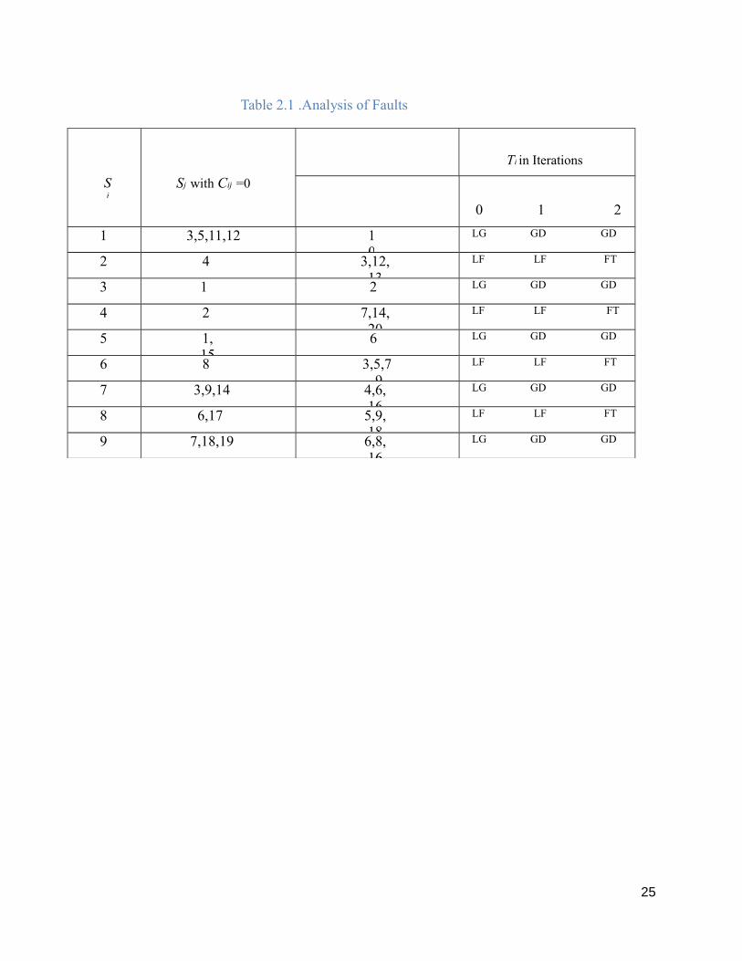
Table 2.1 .Analysis of Faults

Si

Sj with Cij =0 Sj with Cij =1

Ti in Iterations

0 1 2

1 3,5,11,12 10

LG GD GD

2 4 3,12,13

LF LF FT

3 1,

2,

LG GD GD

4 2 7,14,20

LF LF FT

5 1,15

6,

LG GD GD

6 8 3,5,7,9

LF LF FT

7 3,9,14 4,6,16

LG GD GD

8 6,17 5,9,18

LF LF FT

9 7,18,19 6,8,16

LG GD GD

25

CHAPTER 3

PROPOSED MECHANISM

28

3 PROPOSED MECHANISM

3.1 Network model and Fault modelWe assume that sensors are randomly deployed in the interested area which is very dense and all the sensors have a common transmission range. The dark circles in the figure represent faulty sensors and the gray circles are good sensors. There might be a failure occurring in a certain area as illustrated in the figure 2.1. All sensors in this area go out of service[1].As we are depending on majority voting among the sensors, we assume that each sensor node has at least 3 neighboring nodes. Because a large amount of sensors are deployed into the interested area to form a wireless network, this condition can be easily obtained. Each sensor node is able to locate its neighbors within its transmission range via a broadcast/ acknowledge protocol. Faults can occur at different levels of the sensor network [8], such as system software, hardware, physical layer, and middleware.In this mechanism, we focus on hardware level faults by assuming all system software as well as the application software is always fault tolerant. We can categorize the hardware components of sensor nodes into two groups. The first group of hardware level components consists of a storage subsystem, computation engine and power supply infrastructure. The second groups of components are sensors and actuators. The second group is most prone to malfunctioning. We only consider the sensor faults which occur in the second group [8]. Sensor nodes are still capable of receiving, sending, and processing when they are faulty in the algorithm.

Failure Node Working Node

Figure 3.1.Sensor nodes randomly deployed over an area29

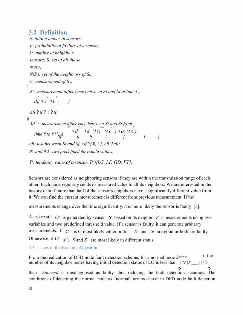
3.2 Definitionn: total n umber of sensors;

p: probability of fa ilure of a sensor;

k: number of neighbo r

sensors; S: set of all the se

nsors;

N(Si): set of the neighb ors of Si;

xi: measurement of S i;ij

d t : measurement differ ence betwe en Si and Sj at time t ,

d t

? x t

? x t

;ij i j

Δtl ? tl ? 1 ? tl;ij

Δd Δtl : measurement differ ence betwe en Si and Sj from

time tl to tl ? 1, Δ

Δtl

? d tl ?1

? d tl

? (xtl ?1

? xtl ?1

) ? (xtl

? xtl

);ij ij ij i j i j

cij: test bet ween Si and Sj, cij ?{ 0, 1}, cij ? cji;

θ1 and θ 2: two predefined thr eshold values;

Ti: tendency value of a sensor, Ti ?{LG, LF, GD, FT};

Sensors are considered as neighboring sensors if they are within the transmission range of each other. Each node regularly sends its measured value to all its neighbors. We are interested in the history data if more than half of the sensor’s neighbors have a significantly different value from it. We can find the current measurement is different from previous measurement. If the

measurements change over the time significantly, it is more likely the sensor is faulty [3].

A test result Cij is generated by sensor Si based on its neighbor Sj ’s measurements using two

variables and two predefined threshold value. If a sensor is faulty, it can generate arbitrarymeasurements. If Cij is 0, most likely either both Si and Sj are good or both are faulty.

Otherwise, if Cijis 1, Si and Sj are most likely in different status.

3.3 Issues in the Existing Algorithm

From the realization of DFD node fault detection scheme, for a normal node Snormal , if the

number of its neighbor nodes having initial detection status of LG is less than

?| N (Snormal) | / 2

? ,

then Snormal is misdiagnosed as faulty, thus reducing the fault detection accuracy. The conditions of detecting the normal node as “normal” are too harsh in DFD node fault detection

30

scheme. Besides, the node fault accuracy of DFD scheme will decrease rapidly when there are not many neighbors of the nodes to be detected or the node’s failure ratio of network is high [4].

31

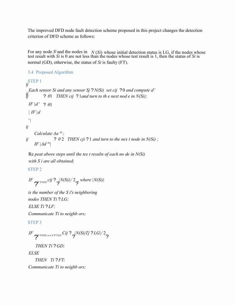
The improved DFD node fault detection scheme proposed in this project changes the detection criterion of DFD scheme as follows:

For any node Si and the nodes in N (Si) whose initial detection status is LG, if the nodes whosetest result with Si is 0 are not less than the nodes whose test result is 1, then the status of Si is normal (GD), otherwise, the status of Si is faulty (FT).

3.4 Proposed Algorithm

STEP 1ij

Each sensor Si and any sensor Sj ? N(Si) set cij ? 0 and compute d t

ijij

IF |d t

| IF |d t |

? θ1

? θ1

THEN cij ? 1and turn to th e next nod e in N(Si);

ij

Calculate Δa Δtl ;ij

IF |Δd Δtl|? θ 2 THEN cji ? 1 and turn to the nex t node in N(Si) ;

Re peat above steps until the tes t results of each no de in N(Si)

with S i are all obtained;

STEP 2

IF ?Sj ? N(Si)

cij ? ?

|N(Si)|/ 2?

, where |N(Si)|

is the number of the S i's neighboring

nodes THEN Ti ? LG;

ELSE Ti ? LF;

Communicate Ti to neighb ors;

STEP 3

IF ?Sj ? N(Si) a n d Tj ? LG

Cij ? ?

|N(Si)Tj ? LG|/ 2?

THEN Ti ? GD;

ELSE

THEN Ti ? FT;

Communicate Ti to neighb ors;

STEP 4If there are no neighbor nodes of S

i

Whose initial detection status is LG, and if the initial detection status T

i of S

i is LG, then set the

status of Si

as normal (GD), otherwise as fault(FT);

STEP 5Check whether detection of the status of all nodes in network is completed or not. If it has been completed, then exit. Otherwise, repeat steps of (1), (2), (3) and (4).

CHAPTER 4

SIMULATION AND RESULTS

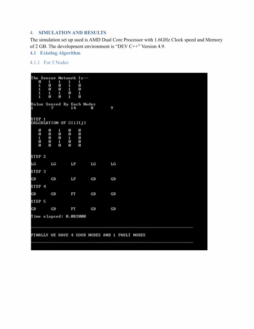
4. SIMULATION AND RESULTS

The simulation set up used is AMD Dual Core Processor with 1.6GHz Clock speed and Memory of 2 GB. The development environment is “DEV C++” Version 4.9.4.1 Existing Algorithm

4.1.1 For 5 Nodes

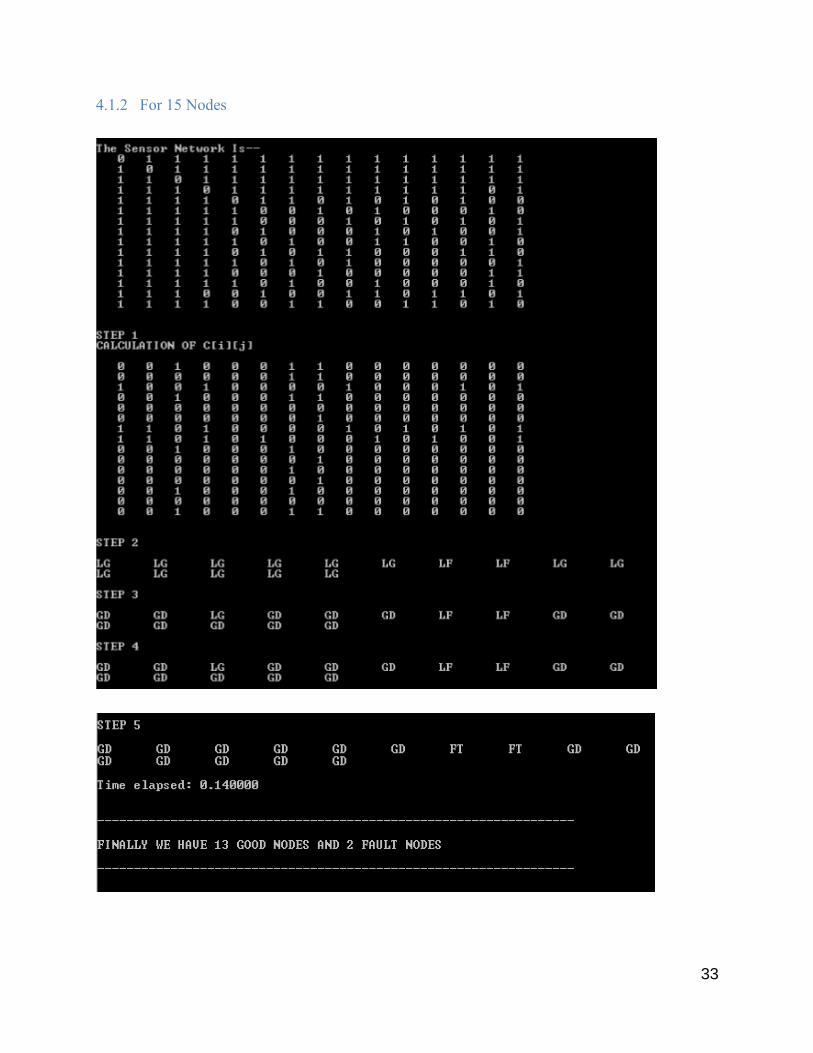
4.1.2 For 15 Nodes

33

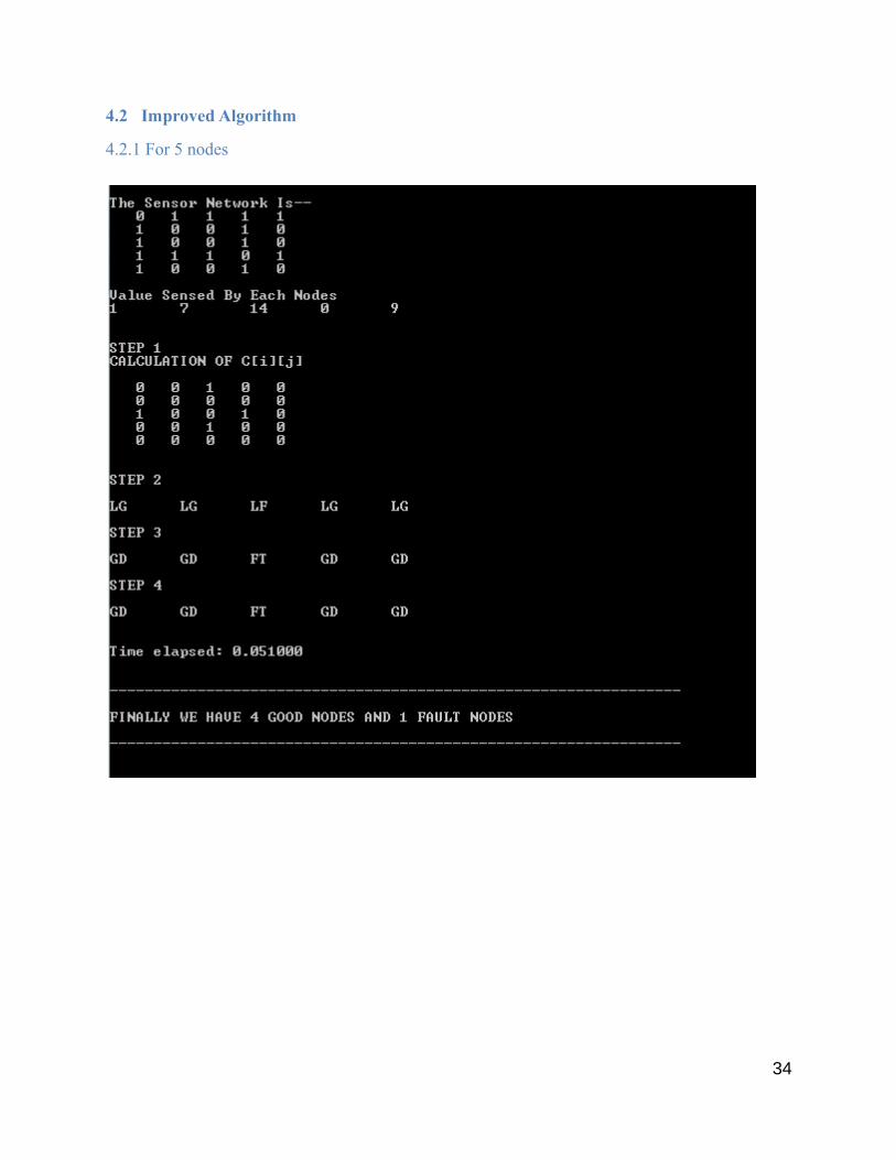
4.2 Improved Algorithm

4.2.1 For 5 nodes

34

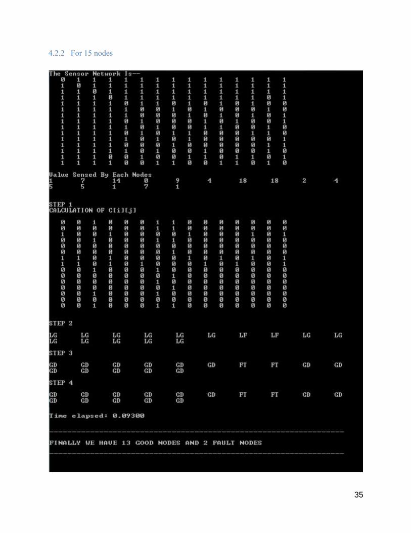
4.2.2 For 15 nodes

35

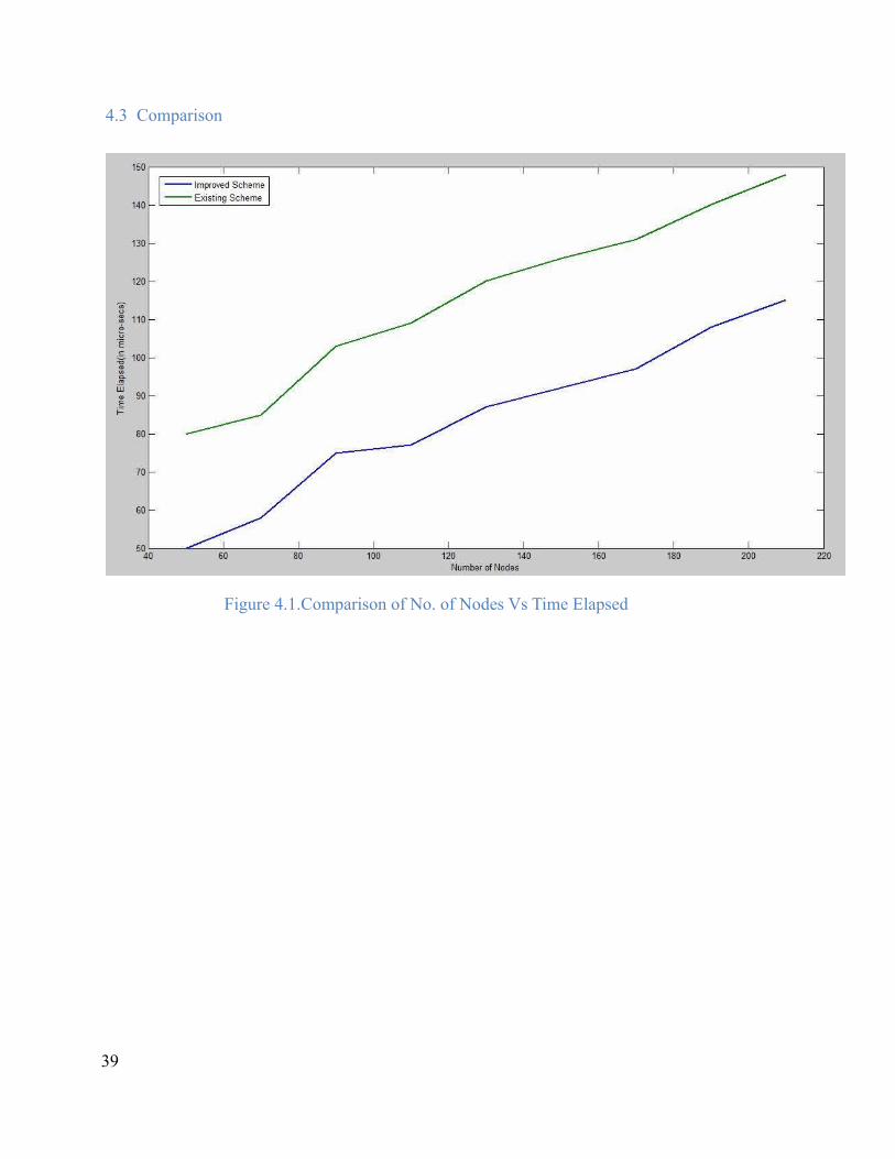
4.3 Comparison

Figure 4.1.Comparison of No. of Nodes Vs Time Elapsed

39

CHAPTER 5

CONCLUSION

40

5. CONCLUSION

5.1 Conclusion

We proposed a distributed localized faulty sensor detection algorithm where each sensor identifies its own status to be either ”good” or ”faulty” and the claim is then supported or reverted by its neighbors as they also evaluate the node behavior. We have shown the simulation results in the form of graphs. By the Simulation results, we conclude that the time consumed by our approach to find out the faulty node is relatively less than the time consumed by the existing scheme.

5.2 Future workIn future we intend to calculate the detection accuracy for the nodes in the Wireless SensorNetwork where detection accuracy depicts the ratio of the number of faulty sensors detected tothe total number of faulty sensors in the network. The time consumed by our approach to find out the faulty node is relatively less. So we want to verify it for larger number of nodes.

41

REFERENCES:

[1] Jinran Chen, Shubha Kher and Arun Somani. Distributed Fault Detection of Wireless Sensor networks, Dependable Computing and Networking LabIowa State UniversityAmes,Iowa .pages75-84,Computer Network,2006.

[2] D. Blough, G. Sullivan, and G. Masson. Faultdiagnosis for sparsely interconnected multiprocessor systems. In In 19th Int. IEEE Symp. on FaultTolerantComputing, pages62–69. IEEE Computer Society, 1989.

[3] F. Koushanfar, M. Potkonjak, and A. Sangiovanni-Vincentelli. On-line fault detection of sensor measurements. In Sensors, 2003. Proceedings of IEEE, pages 974–979 Vol.2,2003.

[4] X. Luo, M. Dong, and Y. Huang. On distributed fault-tolerant detection in wireless sensor networks. IEEE Transactions on Computers, Jan2006.

[5] Akyildiz, I.F.; Su, W.; Sankarasubramaniam, Y; Cayirci, E. Wireless sensor networks:a survey.Computer Networks 2002.

[6] M. Ding, D. Chen, K. Xing, and X. Cheng. Localized fault-tolerant event boundary detection in sensor networks. In Proceedings of IEEE INFOCOM 2005,2005.

[7] F. Koushanfar, M. Potkonjak, and A. Sangiovanni-Vincentelli. Fault-tolerance in sensor networks.In Handbook of Sensor Networks. CRCpress, 2004.

[8] B. Krishnamachari and S. Iyengar. Distributed bayesian algorithms for fault-tolerant event region detection in wireless sensor networks. IEEE Transactions on Computers,53(3):241–250, March 2004.

[9] Mahmood and E. J. McCluskey. Concurrent error detection using watchdog processors- a survey.Computers, IEEE Transactions on, 37(2):160–174, Feb 1988.

[10] S. Marti, T. J. Giuli, K. Lai, and M. Baker. Mitigating routing misbehaviour in mobile ad hoc networks. In MobiCom ’00: Proceedings of the 6th annual international conference on Mobile computing and networking, pages 255–265, New York, NY, USA, 2000. ACM Press.

[11] Perrig, R. Szewczyk, V. Wen, D. E. Culler, andJ. D. Tygar. SPINS: security protocols for sensor netowrks. In Mobile Computing and Networking, pages 189–199, 2001.

42

[12] L. B. Ruiz, I. G. Siqueira, L. B. e Oliveira, H. C. Wong, J. M. S. Nogueira, and A.A. F. Loureiro. Fault management in event-driven wirelesssensornetworks.InMSWiM’04:

[13] Proceedings of the 7th ACM international symposium on Modeling, analysis and simulation of wireless and mobile systems, pages149–156, New York, NY, USA, 2004. ACM Press.

[14] K. Somani and V. K. Agarwal. Distributed diagnosis algorithms for regular interconnected structures. Computers, IEEE Transactions on,41(7):899–906, July 1992.

[15] J. Staddon, D. Balfanz, and G. Durfee. Efficient tracing of failed nodes in sensor networks. In WSNA ’02: Proceedings of the 1st ACM internationalworkshop on Wireless sensor networks and applications, pages 122–130, New York, NY, USA,2002. ACM Press.

[16] S. Tanachaiwiwat, P. Dave, R. Bhindwale, and A. Helmy. Secure locations: routing on trust and isolating compromised sensors in location-aware sensor networks. In SenSys, pages 324–325, 2003.

[17] M. Yu, H. Mokhtar, and M. Merabti, "A survey on Fault Management in wireless sensor network," inProceedings of the 8th Annual PostGraduate Symposium on The Convergence of Telecommunications, Networking and Broadcasting Liverpool, UK,2007.

[18] S. Marti, T. J. Giuli, K.Lai, and M. Baker, "Mitigating routing misbehaviour in mobile ad hoc networks," in ACM Mobicom, 2000, pp. 255-265.

[19] F. Koushanfar, M. Potkonjak, and A. SangiovanniVincentelli, "Fault tolerance techniques in wireless ad-hoc sensor networks," UC Berkeley technical reports 2002.

[20] W. L. Lee, A. Datta, and R. Cardell-Oliver, "WinMS: Wireless Sensor Network- Management System, An Adaptive Policy-Based Management for Wireless Sensor Networks," School of International Journal of Wireless & Mobile Networks (IJWMN) Vol.2, No.4, November 2010.

43

[21] T. Clouqueur, K.Saluja, and P. Ramanathan, "Fault Tolerance in CollaborativeSensor Networks for Target Detection," in IEEE Transactions on Computers, 2004, pp.320-333.

[22] G. Gupta and M. Younis, "Fault-Tolerant Clustering of Wireless SensorNetworks," in Proceedings of the IEEE WCNC 2003 New Orleans, Louisiana, 2003.

44