a strategy for the integration of production planning and scheduling in refineries under uncertainty

PROCESS SYSTEMS ENGINEERING Chinese Journal of Chemical Engineering, 17(1) 113 127 (2009)

A Strategy for the Integration of Production Planning and Scheduling in Refineries under Uncertainty*

LUO Chunpeng ( ) and RONG Gang ( )**State Key Lab. of Industrial Control Technology, Institute of Cyber System and Control, Zhejiang University, Hang-zhou 310027, China

Abstract A strategy for the integration of production planning and scheduling in refineries is proposed. This strat-egy relies on rolling horizon strategy and a two-level decomposition strategy. This strategy involves an upper level multiperiod mixed integer linear programming (MILP) model and a lower level simulation system, which is ex-tended from our previous framework for short-term scheduling problems [Luo, C.P., Rong, G., “Hierarchical ap-proach for short-term scheduling in refineries”, Ind. Eng. Chem. Res., 46, 3656 3668 (2007)]. The main purpose of this extended framework is to reduce the number of variables and the size of the optimization model and, to quickly find the optimal solution for the integrated planning/scheduling problem in refineries. Uncertainties are also con-sidered in this article. An integrated robust optimization approach is introduced to cope with uncertain parameters with both continuous and discrete probability distribution. Keywords refinery, planning and scheduling, optimization model, simulation system

1 INTRODUCTION

To compete successfully in international markets, oil refineries are concerned with improving the plan-ning and scheduling of their operations to achieve better economic performance. Many progresses have been achieved on planning and scheduling in refiner-ies [1 3], and commercial softwares, such as RPMS, PIMS and ORION, for refinery production planning and scheduling have facilitated the development of general production plans and schedules of the whole refinery. Linear programming is a good technique for production planning of refineries. However the short-term scheduling problem is still one of the most challenging problems in operational research due to the complexity of the scheduling operations and the corresponding process models. In addition, the inte-gration of planning and scheduling has received less attention because of the major challenges toward dealing with the different time scales and the problem size of the resulting optimization model.

To meet the challenge in the short-term schedul-ing, many scheduling models and solution strategies, such as scheduling models with discrete time formula-tion, scheduling models with continuous-time formu-lation, decompose strategies, heuristic algorithms, and simulation and expert systems, have been proposed in literature [1 13]. When a model is described with dis-crete time, the time slot duration must be short enough to honor all the operation rules and the variables dur-ing the whole scheduling horizon will increase dra-matically. Pinto and Joly [9] had defined a time slot duration of 15 minutes for crude oil scheduling prob-lems, which generated a discrete time mixed integer optimization model with 21504 binary variables in a

3 4 days horizon. They pointed out that the solution of such a problem is far beyond the capabilities of the current optimization technology. The continuous-time modeling is particularly suitable for scheduling prob-lems with activities ranging from a few minutes to several hours. Because of the possibility of eliminat-ing a major fraction of the inactive event-time interval, the resulting mathematical programming problems are usually of much smaller sizes and require less compu-tational efforts for their solution [2, 3, 6]. However, due to the variable nature of the timings of the events, it becomes more challenging to model the scheduling processes and the continuous-time approach may lead to mathematical models with more complicated struc-tures compared with their discrete-time counterparts.

Some other authors have resorted to intelligent simulation systems to deal with scheduling problems. Paolucci and Sacile [11] used a simulation-based deci-sion support system (DSS) to improve the effective-ness of the decisions on allocating crude oil supply to port and refinery tanks. Chryssolouris and Papakostas [12] used an integrated simulation-based approach to evaluate the performance of short-term scheduling with tank farm, inventory and distillation management. The use of simulation model to provide decision sup-port can allow the application of public domain of heuristic knowledge, support what-if analysis and be able to evaluate the performance of alternative solu-tions. But simulation systems rely on the user to spec-ify the independent variables, i.e., flows into and out of a unit over time. The simulator can then calculate the dependent variables such as a tank’s holdup and quality at each time interval. The values of those in-dependent variables are mainly dependent on sched-uler’s experience and can’t ensure optimal schedules.

Received 2008-05-05, accepted 2008-08-19.

* Supported by the National Natural Science Foundation of China (60421002) and the National High Technology R&D Program of China (2007AA04Z191).

** To whom correspondence should be addressed. E-mail: [email protected]

Chin. J. Chem. Eng., Vol. 17, No. 1, February 2009 114

Although many progresses have been achieved on planning and scheduling in refineries, the integra-tion of planning and scheduling has received less at-tention. Two of the major challenges towards this in-tegration are dealing with the different time scales and with the problem size of the resulting optimization model [14 17].

Regarding the time representation, one approach is to define a very large scheduling problem that spans the whole planning horizon and, to define longer lengths for future time periods to yield a formulation where the immediate future includes more details than the distant future. This approach always generates a model that can not be solved in the full space due to its size and that some type of decomposition is re-quired [14, 15]. The second approach is to define an aggregate planning problem and a detailed scheduling problem with equivalent horizon, and information is passed from the planning model to the scheduling model [14, 16]. A third method for dealing with the different time scales is to use a rolling horizon ap-proach where only a subset of the planning periods include the detailed scheduling decisions with shorter time increments. The detailed planning/scheduling period moves as the model is solved in time [14, 17]. When such a planning/scheduling model is solved in real time, the first planning period is often a detailed scheduling model while the future planning periods include only planning decisions and this approach is mainly used in this study.

Because of the challenge in the computation of the integrated planning/scheduling problem, a frame-work is introduced in this article. This framework is an extension of our previous study, which involves two decision levels for short-term scheduling prob-lems in refineries: an optimization model at the upper level and a simulation system at the lower level. The main purpose of the approach is to reduce the binary variables and the size of the optimization model caused by the representation of multipurpose tanks in refineries and operation rules for material movements. The optimization model is used to decide when, how long, and how much an operation (operation mode) is active and, also, to determine how many materials (raw materials, intermediate materials, and final products) are produced and consumed by the opera-tions. In this optimization model, only operation modes of processing units, blenders, and pipelines are considered. Although this model is based on discrete time formulation, we use the methods mentioned by GÖthe-Lundgren and Lundgren [4] to extend the model and allow the start and end of each operation mode at any point in a time slot. Another characteristic of the optimization model is that only aggregate tanks are used, and that each kind of material [2, 3, 6] has only one aggregate tank. The details of material movements between all actual units (including indi-vidual tanks) will be determined in the simulation system at the lower level. The simulation system uses some heuristics and rules to arrange actual tanks to receive/send materials with logic operation constraints

(operation rules) on respective tanks. The maximum storage capacities of aggregate tanks can be violated in the optimization model, and this strategy is used to model the multipurpose tanks, which can hold differ-ent materials in different operation modes. The simu-lation system uses a heuristic to try to eliminate the extra capacity requirements of these aggregate tanks. The iteration procedure between the upper level and the lower level can be used to find optimal solution under updated aggregate storage capacities. With the cooperation of the simulation system, the upper level optimization model only needs to make macro deci-sions, and the time slot does not need to be short enough to honor all the operation rules. Just for this reason, we believe that the upper level model can be easily transformed to an integrated planning/scheduling optimization model, and that the simulation system can still be a good tool for the detailed decision-making during the scheduling horizon.

Uncertainties are also considered in our integrated planning/scheduling model. Generally, stochastic mod-els under uncertainty can be divided into two catego-ries depending on whether it follows the scenario-based framework. When the uncertain parameters follow continuous probability distribution, one usually gen-erates a finite set of scenarios, from sampling or a dis-crete approximation of the given distributions, to rep-resent the probability space [18]. As the number of uncertain parameters increases, more scenarios must be considered, which results in a much larger problem. This main drawback that limits the application of these approaches is to solve practical problems with various uncertain parameters. Stochastic models not following scenario-based framework have also been applied to scheduling problems, and probabilistic (chance) programming, fuzzy mathematical program-ming, probabilistic programming, and flexible pro-gramming are important approaches of non-scenario- based framework [19].

In this article, we integrate the robust optimiza-tion approach presented by Janak et al. and Leung et al., to cope with the uncertain parameters with both continuous and discrete probability distribution re-spectively [20, 21].

2 ARCHITECTURE OF THE STRATEGY

In this study, the hierarchical approach of our previous framework for short-term scheduling in re-fineries is extended, which includes a mathematical programming model at the upper level and a simula-tion system at the lower level [22]. The upper level optimization model is now changed to an integrated robust planning/scheduling model. A time representa-tion called rolling horizon mode is adopted to address the integrated planning/scheduling optimization strat-egy in refineries. The planning horizon (1 to 3 months) is divided into a certain number of planning periods (weeks). Only the first planning period includes the de-tailed scheduling decisions with shorter time increments


(days), and only those decisions belonging to the first planning period are passed to the simulation system at the lower level. At the end of the first planning period, the state of the system is updated, and the computa-tional cycle is repeated with the horizon advancing one period by one period.

The mathematical scheduling model in the first planning period is based on discrete time formulation with 1 day increment for each scheduling period. This scheduling model is used to decide sequencing and timing of the operation modes of units and to determine the quantities of materials consumed/produced by each operation mode of a unit. Although this is a schedul-ing model, it does not consider the operation details of each individual tank. Only aggregate tanks are con-sidered in this model, and an aggregate tank is used only for one kind of material. And the operation rules related to material movements for each individual tank are not considered in this model. The storage capacity of an aggregate tank is the sum of the storage capaci-ties of individual tanks storing the same material.

It is well-known that there exits multipurpose tanks in refineries, and they can be used to store dif-ferent materials when their operation modes are changed. An aggregate tank may possess some multi-purpose tanks, so the storage capacity of an aggregate tank may change depending on which operation modes the multipurpose tanks will be in.

To model the alterable storage capacity of each aggregate tank, the maximum storage capacities of aggregate tanks can be violated by using some slack variables which are punished by penalties in the mathematical model. And the value of each slack variable, which is called the extra capacity require-ment of an aggregate tank, represents the degree to which the current maximum storage capacity of a cor-responding aggregate tank cannot satisfy the demands of production.

The planning model beyond the first planning period is similar to the scheduling model. The main difference is that the planning period (1 week) is longer than the scheduling model (1 day), and the planning model is only used to determine which op-eration is active and how long an operation is active during each period. So the tight constraints, such that each unit can at most be in one mode during a period, are relaxed in the planning model. And, some opera-tion details considered in the scheduling model, such as modeling the changeover of operation modes be-

tween two adjacent periods, and modeling the variety of the charge size of each unit between two adjacent periods, are ignored in the planning model. In the planning model, aggregate tanks are the same as those in the scheduling model, and the maximum storage capacities of aggregate tanks can also be violated.

Because slack variables are used in the upper level optimization model to represent the extra storage capacity requirements of aggregate tanks, one impor-tant role of the simulation system at the lower level is trying to eliminate the extra capacity requirements by adjusting the operation modes of the multipurpose tanks within some aggregate tanks that have redundant capacities. Once the upper level model finds an opti-mal solution without extra storage capacity require-ments, another important role of the simulation system is to determine detailed operations for each individual tank with operation rules considered. These decisions involve arranging the sequence and the time point that each individual tank receives/sends materials. Some heuristics are used in the simulation system to deal with these tasks.

The strategies, involving the mathematical rep-resentation of multipurpose tanks and the operation rules for material movements related to each individ-ual tank are ignored in the mathematical model, can reduce a large number of binary variables and the size of the integrated planning/scheduling model. This can help the model to find the optimum solution within a reasonable time.

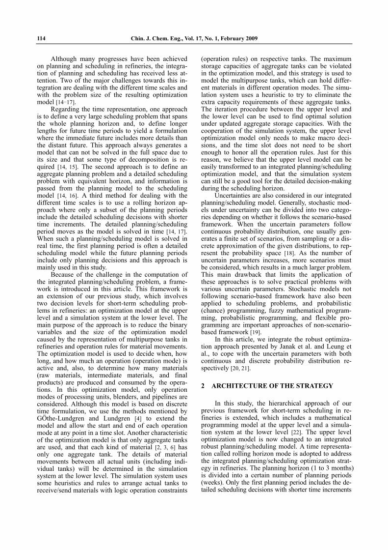
The solution strategy for the integrated planning/ scheduling decisions of refineries involves an iteration procedure between the integrated planning/scheduling optimization model and the simulation system. The iteration procedure is shown in Fig. 2. When the inte-grated planning/scheduling optimization model finds an optimal solution, the variables in the first planning period, which are scheduling decisions, are taken as inputs in the simulation system at the lower level. The lower level then first tries to eliminate the extra capac-ity requirements by adjusting the operation modes of the multipurpose tanks within some aggregate tanks that have redundant capacities. When the simulation system adjusts the operation modes of some multi-purpose tanks, the storage capacities of the corre-sponding aggregate tanks will be changed. Then the updated storage capacities will be feed back to the mathematical model at the upper level, and the inte-grated planning/scheduling optimization model will be

Figure 1 Time representation of our approach


recalculated to find the new optimal solution. The variables in the first planning period of this new opti-mal solution are again taken as inputs in the simula-tion system, and then the simulation system try to eliminate the new extra capacity requirements. So, there is an iterative link between the upper lever and the lower level.

If the simulation system at the lower level cannot find redundant storage capacities, the maximum stor-age capacity constraints at the upper level must be changed to hard constraints that cannot be violated. The optimization model will be recalculated with hard constraints. The iteration procedure of our approach is shown in Fig. 2 and the termination conditions of the iteration procedure can be referred from our previous work [22].

After the termination of the iteration procedure, if an optimal solution is found, the simulation system will continue to use heuristics to determine the de-tailed material movements related to each individual tank in the first planning period.

Because rolling horizon mode is adopted, only the first planning period includes the detailed sched-uling decisions and only these decisions belonging to the first planning period are passed to the simulation system at the lower level. The extra capacity require-ments beyond the first planning period show the shortage of the storage capacities in the future, but they will not be inputted to the simulation system in the current time. When the horizon advances, they will

be dealt with one period by one period. Since our upper level model is for long-term

planning/scheduling problem, its uncertainty is also considered. In this article, properties for components entering blending units are uncertain parameters with continuous probability distribution, and demands for final products in the scheduling horizon are uncertain parameters with discrete probability distribution. The integrated planning/scheduling model with these un-certain parameters is converted to determinative model by integrating the robust approaches proposed by Janak et al. and Leung et al [20, 21]. The approach of Janak et al. can avoid enumerating scenarios for uncertain parameters following continuous probability distribution, but it has the difficulty of dealing with uncertain parameters following discrete probability distribution [20]. However, the approach of Leung et al. can deal with uncertain parameters following discrete probability distribution by enumerating scenarios [21]. In this article, we integrate the robust optimization approach presented by Janak et al. and Leung et al. to cope with the uncertain parameters with both con-tinuous and discrete probability distribution.

3 AN OVERVIEW OF ROBUST OPTIMIZATION

3.1 Scenario-based robust optimization

The robust optimization, presented by Leung et al.,

Figure 2 Iteration procedure of our approach


integrates a goal-programming formulation with a scenario-based description of input data [21]. The model generates a series of solutions that are progres-sively less sensitive to the realizations of input data from a set of scenarios.

Let x be a vector of the design variables that cannot be adjusted once a specific realization of the data has been observed, and let y be a vector of control variables that are subject to adjustment once uncertain parameters are observed. Then the form of their robust optimization model is as follows:

T Tmins.t.

, 0

f x d yAx gBx Cy ex y

(1)

In this model, the first equality is structural con-straint whose coefficients are fixed and free of noise, whilst the second equality is control constraint whose coefficients are subject to noise. The set of scenarios involved is CS {1, 2, 3, ···, sc}. Under each scenario sc SC, the coefficients associated with the control constraints will become

c c c c, , ,s s s sd B C e with fixed

probability cB,sP , which represents the probability that

scenario sc happens and has c

c

B, 1ss

P . The optimal

solution of this model will be robust with respect to optimality if it remains “close” to optimality for any realization of scenarios. This is called as solution ro-bustness. The solution is also robust with respect to feasibility if it remains “almost” feasible for any re-alization of sc. The trade-off between solution robust-ness and model robustness should be determined through use of the multiple-criteria decision-making concept. The robust optimization model is formulated to measure this trade-off. The robust optimization model based on the mathematical programming prob-lem 1 is formulated as follows:

c c

c C

c c c c c c

c C c C c C

c c c

c c c c c

c

TB,

B, B, B,

T

c C

c C

min

s.t.

for all

, 0 for all

s ss S

s s s s s ss S s S s S

s s s

s s s s s

s

x P

P P w P

x y s S

s S

f

d y

Ax gB C e

x y

(2)

where variable cs is used to measure the infeasibility

allowed in the control constraints under scenario sc. Term

c c c c c c

c C c C c C

B, B, B,s s s s s ss S s S s S

P P P in

the objective is used to measure the solution robust-

ness, and term c c

c C

B,s ss S

P is used to measure the

model robustness. The sensitivity of the solution to the realization of uncertainty data is controlled by pa-rameter , and the trade-off between solution robust-ness and model robustness is controlled by weight w.

3.2 Non-scenario-based robust optimization

Janak et al. assumed that the uncertainty may arise from both the coefficients and the right-hand-side parameters of the inequality constraints, and the un-certainty may also arise from the coefficients of ob-jective function [20]. Thus, the feasibility of the fol-lowing inequality is concerned.

Tmins.t.

lm m lm

b x e

x x x

c xAx d

(3)

where lmb and le are the “true” values of the uncer-tain parameters, l is the index of the uncertain inequal-ity, m is the index of the variables.

Assuming that the true values of the uncertain parameters are obtained from their nominal values by random perturbations:

1

1lm lm lm

l l

b b

e e (4)

where lm and l are independent random variables in the interval [ 1,1] , blm and el are the nominal val-ues of the uncertain parameters, and 0 is a given (relative) uncertainty level.

In this situation, solution x is called robust if it satisfies the following:

(i) x is feasible for the nominal problem, and (ii) the probability of violation of the uncertain

inequality with an error is at most k:

max[1, ]Pr lm m l lm

b x e e k (5)

where 0 is a given feasibility tolerance and is introduced to allow a small amount of infeasibility in the uncertain inequality, and 0k is a given reliabil-ity level. Thus, k represents the probability of viola-tion of constraint l. Substituting the expressions for the true values of the uncertain coefficients given (4) (i.e., lmb , le ) and rearranging the terms, we can re-write (5) as follows:

Pr

max[1, | |]

lm m lm

lm lm m l l lm

b x e

b x e e k (6)

When the probability distribution function for the


uncertainty term lm lm m l lm

b x e in (6) is known,

it is possible to obtain a more accurate estimation of the probability measures. This is done by using the definition of probability distribution function of and the following relationship:

( ) Pr 1 Pr 1F k (7)

The final form of the deterministic constraint (or robust counterpart problem) is simply determined us-ing the inverse distribution function of the random variable . Let

1, , (1 )lm m lf b x e F k (8)

then we can get the deterministic constraint: , , max 1,lm m lm m l l l

mb x f b x e e e . (9)

4 INTEGRATED PLANNING/SCHEDULING MODEL

The proposed model divides the planning horizon H (1 3 months) into periods of length H1 (1 week) where production is planned using both known and estimated demands. The first planning period of the time horizon is divided into time intervals of lower length H2 (1 day). The model is to be rerun every pe-riod H1 as forecasts become real orders. In the model, demands for some final products in the first planning period are random parameters with discrete probabil-ity distribution, which represents the fluctuation of arrival time of vehicles that transport products. How-ever, the properties for components entering the blend-ers are all random parameters with continuous prob-ability distribution during the whole planning horizon.

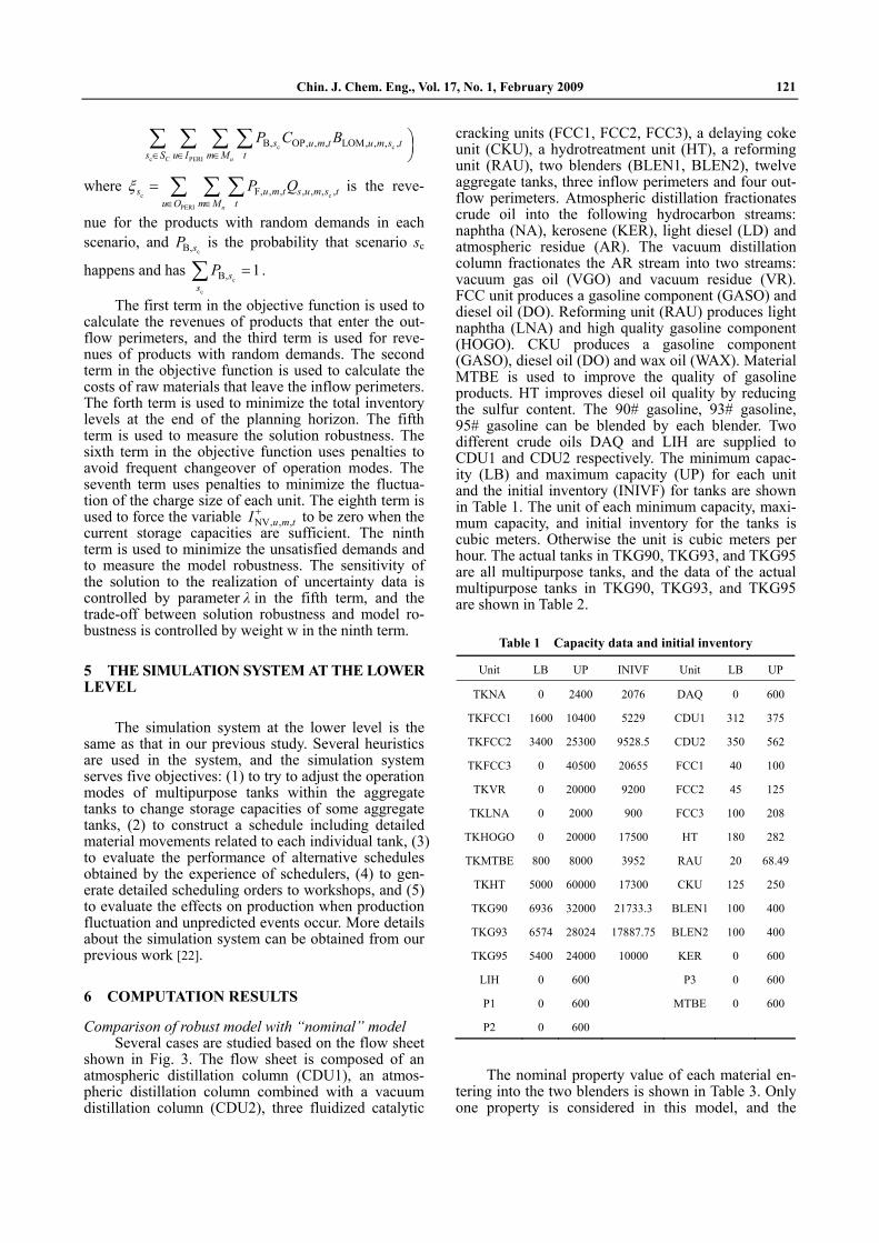
The optimization model is a MILP model based on discrete time. The flow sheet of a refinery studied is the same as our previous work, as shown in Fig. 3. The figure consists of a set of rectangles/triangles that represent the units/tanks in the plant and “connec-tions” which represent the flow paths between equip-ments. The small squares connected to the equipment by short lines are the “ports” where flow enters or leaves the equipment. The pentagons represent the “perimeter” (equivalent to pipelines) through which materials entering/leaving the plant. The ports of pe-rimeters are not shown in the figure for simplification. Supply orders or demand orders can be defined on the perimeters. The description of the flow sheet in Fig. 3 is based on the works of Kelly and on Honeywell Process Solutions called “Honeywell Production Scheduler”, and the modeling data is provided by a refinery of PetroChina where “Honeywell Production Scheduler” has been implemented [23, 24].

4.1 Constraints of the scheduling model in the first planning period

Some constraints are similar to our previous study, it is not presented here and more details can be obtained from our previous work [22] and Appendix A. The following constraints are only the important con-straints that can help to understand the strategies adopted in this study.

Material balance equation for each tank (prod-ucts with uncertain demands):

c c cNV, , , , NV, , , , 1 , , , , , , ,u m s t u m s t s u m t s u m s tI I Q Q

Ku T , S,us I , S,us O , St T , c Cs S (10)

c c

ONM, , ,

, , , , , , , , , , ,( , , ) s u m

s u m s t s u m s u m s ts u m C

Q Q

Figure 3 Simplified flow sheet of a refinery


,u U St T , S,us O , um M , c Cs S (11)

Because the demands for products are uncertain pa-rameters with discrete probability distribution in the scheduling model, which are caused by the fluctuation of the arrival time of vehicles, these products leaving the outflow ports of their tanks will fluctuate accord-ing to the change of demands. So the inventory for these products will be different in different scenario sc. In this model, we assume the flows that entering these product tanks are design variables, which cannot be adjusted once a specific realization of the uncertain data has been observed. This means that the fluctua-tion of demands will not affect the production of these products and only affect the inventory of these prod-ucts. The total scenarios are generated according to the combination of the realization of all uncertain pa-rameters with discrete probability distribution. The inventory of these products at the end of time slot t in scenario sc equals to the inventory at the end of time slot 1t in scenario sc plus the amount of the flows entering the unit during time slot t minus the amount of flows leaving the unit during time slot t in scenario sc, as shown in (10). Constraint (11) relates the volu-metric flow of outflow port s with every flow that leaves that port in each scenario.

Storage capacity constraint: low upNV, NV, , , NV,uu u m tI I I Au T , St T (12)

c

low upNV, NV, , , , NV,u u m s t uI I I

Au T , St T , c Cs S (13) Softened product storage capacity constraint:

upNV, , , NV, NV, , ,u m t u u m tI I I TAu V , St T (14)

c

upNV, , , , NV, NV, , ,u m s t u u m tI I I

TAu V , St T , c Cs S (15) Constraints (12) and (13) specify that the minimum and maximum capacity of each aggregate tank must be satisfied if there are no other storage capacities that can be adjusted to extend the current storage capacity. Otherwise the maximum storage capacity can be vio-lated as shown by (14) and (15). Constraints (13) and (15) are used for products with random demands.

Product property constraints:

S, ONM, , ,

lowRO, , , , , , , ,

, , , , , , , , ,( , , )u s u m

s u m p t F u m t

s u m s u m t s u m ps I s u m C

P Q

Q P

S, ONM , , ,

, , , , , , , , ,( , , )

upF, , ,RO, , , , ,

u s u m


u m ts u m p t

Q P

P Q

S, LEN S, , , ,u us O u B m M t T p P (16) These constraints are used to blenders only. The

properties of the product leaving the outflow port

(each blender only has one outflow port) can be di-rectly predicted by using a volumetric average, and, constraint (16) specifies that property p of the flow leaving the outflow port must satisfy the minimum and maximum specifications. In this article, we as-sume that the properties of the flows entering the blenders are random parameters with continuous probability distribution. The blending index for each of the different nonlinear qualities is used to convert each of the nonlinear qualities to a linear index that may be blended linearly by volume.

Let the reliability level for this uncertain con-straint be k, and assume that the true value of each uncertain property of component is obtained from their nominal values by random perturbations, which is shown as follows:

S, ONM, , ,

S, ONM, , ,

, , , , , , , , ,( , , )

upF, , ,RO, , , , ,

, , , , , , , , ,( , , )

lowRO, , , , , F, , ,

, ,, , ,

Pr

Pr

1

u s u m

u s u m


u m ts u m p t


s u m p t u m t

s us u m p

Q P

P Q k

Q P

P Q k

P , , , ,m p s u m pP (17)

where all , , ,s u m p are independent random variables in the interval [ 1,1] , all , , ,s u m pP are the nominal values of the uncertain parameters and, 0 is a given (relative) uncertainty level. And let:

S, ONM, , ,

, ,

, , , , , , , , , , , ,( , , )u s u m

u m p

s u m p s u m s u m t s u m ps I s u m C

Q P

Then the deterministic robust counterpart problem of (17) is (18).

S, ONM, , ,

S, ONM, , ,

, , , , , , , , ,( , , )

up, , , , , , , , ,F, , ,RO, , , , ,

, , , , , , , , ,( , , )

lowRO, , , , , F, , ,

,u s u m

u s u m


s u m s u m t s u m pu m ts u m p t


s u m p t u m t

Q P

Q PP Q f

Q P

P Q , , , , , , , , ,

S, LEN S

,

, , , ,s u m s u m t s u m p

u u

Q Pf

s O u B m M t T p P (18)

where , ,

1( ) 1u m p

f F k and , ,

1u m p

F is the inverse

probability distribution function of , ,u m p . Product supply and demand constraint:

LOM, , , LOM, , , , , , , ,

S, ERI, ,u m t u m t s u m t u m t

u u

B B Q Ds I u P m M (19)

c c c cLOM, , , , LOM, , , , 1 , , , , , , ,

S, ERI c C, , ,u m s t u m s t s u m s t u m s t

u u

B B Q D

s I u P m M s S (20)


, , , , , S, ERI, , ,s u m t u m t u uQ O s O u P m M (21)

The orders defined on the “perimeter” units specify quantities of demands/supplies and the time demands/ supplies. An inflow perimeter has only one outflow port that supplies materials to the plant, and an out-flow perimeter has only one inflow port that receives products from the plant. The different operation modes defined on perimeters represent the different grades of products or different raw materials trans-ferred in these modes. In our model, the demand for each product in each time slot may not be able to be satisfied, and the variables BLOM,u,m,t and

cLOM, , , ,u m s tB are used to represent the total demands that can’t be satisfied at the end of time slot t. They are equal to the total demands that can’t be satisfied at the end of 1t plus the demand needed in time slot t minus the flows transported to customers, as shown in (19) and (20). Constraint (21) ensures that the volumetric flows leav-ing perimeter u during a time slot equal the raw mate-rials supplied in that time slot, and it is used for the inflow perimeter. Constraint (20) is used for products with random demands, and constraint (22) is used to relate the volumetric flow of inflow port s with every flow that enters the port of these outflow perimeters in each scenario.

c c

ONM, , ,

, , , , , , , , , , ,( , , )

ERI S S,, , ,s u m

s u m s t s u m s u m s ts u m C

u u

Q Q

u P t T s I m M (22)

4.2 Constraints of the planning model beyond the first period

The time period in the planning model is 1 week. We assume that the random demands in the first plan-ning period will at most influence the production to the end of the second planning period. So the inven-tory for these products with random demands will be design variables at the end of the second period, which cannot be adjusted once uncertain demands have been observed. Thus, Constraint (10) is changed to:

c cNV, , , NV, , , , 1 , , , , , , ,

K S, S, P c C, , , ,u m t u m s t s u m t s u m s t

u u

I I Q Q

u T s I s O t T s S (23)

where NV, , ,u m tI is the inventory at the end of the sec-ond period, and

cNV, , , , 1u m s tI is the inventory at the end of the first planning period in each scenario.

In the planning model, the maximum capacity of each aggregate tank also can be violated using soft constraints as (12). However, the extra capacity re-quirements beyond the first planning period are not adjusted by the simulation system in the current time, and they will be adjusted one period by one period as the horizon advances. To ensure that the solution be-yond the first planning period is as feasible as possible, the maximum capacity of tank farms that the aggregate tanks belong to cannot be violated, shown as follows:

c

low upNV, NV NV, , , , NV,

A P c C A, , ,

f ,u,m,t u m s t fu u

I I I I

u F t T s S f F (24) The demands beyond the first planning period

will be unknown and be estimated, and the estimated minimum and maximum demands for each product are defined on the outflow perimeters. Constraints (19) (21) are changed as follows:

low up, , , , , , ,

S, ERI P, , ,u m t s u m t u m t

u u

D Q Ds I u P t T m M (25)

c c c

low up, , , , , , , , , ,

S, ERI P c C, , , ,u m s t s u m s t u m s t

u u

D Q D

s I u P m M t T s S (26) low up, , , , , , ,

S, ERI P, , ,u m t s u m t u m t

u u

Q Q Os O u P t T m M (27)

Constraint (26) is only used in the second period. In the planning model, detailed operational rules

considered in the scheduling model are ignored. For example, constraints, such as modeling the change-over of operation modes between two adjacent periods, modeling the variety of the charge size of each unit between two adjacent periods, and that each unit can at most be in one operation mode during one period, can be ignored to allow more than one operation mode during one planning period. Finally, constraints (12), (14), (18), (23) (27), as well as constraints (A-1) (A-4), (A-9), (A-10) in Appendix A, constitute all the planning constraints beyond the first period.

4.3 Objective function

The main objective of the integrated scheduling/ planning problem is to maximize the profits of prod-ucts and minimize all kind of penalties. The objective function is as follows:

PERI

PERI

c c

C PERI

H K

c c cc

c Cc C

TU

F, , , , , ,

Q, , , , , ,

B, F, , , , , , ,

INV, NV, , ,

B,B,

LSM, , M, , ,

maxu

u

c u

u m t s u m tu O m M t

u m t s u m tu I m M t

s u m t s u m s ts S u O m M t

u u m tt T u T

s s ss s Ss S

u m u m tu m N t

P Q

C Q

P P Q

C I

PP

P S

TU TA

PERI

LT, QF, , LI, NV, , ,

OP, , , LOM, , ,u

u u t u u m tu N t u V t

u m t u m tu I m M t

P T P I

w C B


c c

c C PERI

B, OP, , , LOM, , , ,u

s u m t u m s ts S u I m M t

P C B

where c c

PERI

F, , , , , , ,u

s u m t s u m s tu O m M t

P Q is the reve-

nue for the products with random demands in each scenario, and

cB,sP is the probability that scenario sc

happens and has c

c

B, 1ss

P .

The first term in the objective function is used to calculate the revenues of products that enter the out-flow perimeters, and the third term is used for reve-nues of products with random demands. The second term in the objective function is used to calculate the costs of raw materials that leave the inflow perimeters. The forth term is used to minimize the total inventory levels at the end of the planning horizon. The fifth term is used to measure the solution robustness. The sixth term in the objective function uses penalties to avoid frequent changeover of operation modes. The seventh term uses penalties to minimize the fluctua-tion of the charge size of each unit. The eighth term is used to force the variable NV, , ,u m tI to be zero when the current storage capacities are sufficient. The ninth term is used to minimize the unsatisfied demands and to measure the model robustness. The sensitivity of the solution to the realization of uncertainty data is controlled by parameter in the fifth term, and the trade-off between solution robustness and model ro-bustness is controlled by weight w in the ninth term.

5 THE SIMULATION SYSTEM AT THE LOWER LEVEL

The simulation system at the lower level is the same as that in our previous study. Several heuristics are used in the system, and the simulation system serves five objectives: (1) to try to adjust the operation modes of multipurpose tanks within the aggregate tanks to change storage capacities of some aggregate tanks, (2) to construct a schedule including detailed material movements related to each individual tank, (3) to evaluate the performance of alternative schedules obtained by the experience of schedulers, (4) to gen-erate detailed scheduling orders to workshops, and (5) to evaluate the effects on production when production fluctuation and unpredicted events occur. More details about the simulation system can be obtained from our previous work [22].

6 COMPUTATION RESULTS

Comparison of robust model with “nominal” model Several cases are studied based on the flow sheet

shown in Fig. 3. The flow sheet is composed of an atmospheric distillation column (CDU1), an atmos-pheric distillation column combined with a vacuum distillation column (CDU2), three fluidized catalytic

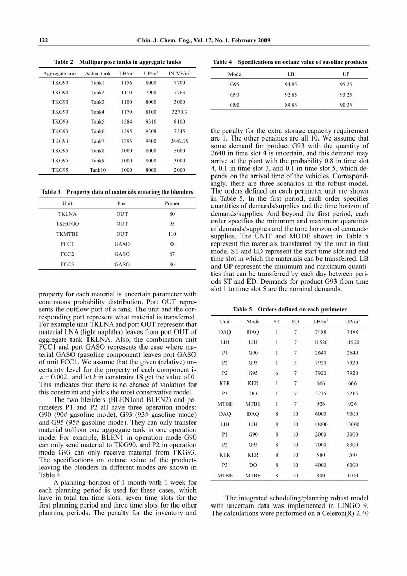
cracking units (FCC1, FCC2, FCC3), a delaying coke unit (CKU), a hydrotreatment unit (HT), a reforming unit (RAU), two blenders (BLEN1, BLEN2), twelve aggregate tanks, three inflow perimeters and four out-flow perimeters. Atmospheric distillation fractionates crude oil into the following hydrocarbon streams: naphtha (NA), kerosene (KER), light diesel (LD) and atmospheric residue (AR). The vacuum distillation column fractionates the AR stream into two streams: vacuum gas oil (VGO) and vacuum residue (VR). FCC unit produces a gasoline component (GASO) and diesel oil (DO). Reforming unit (RAU) produces light naphtha (LNA) and high quality gasoline component (HOGO). CKU produces a gasoline component (GASO), diesel oil (DO) and wax oil (WAX). Material MTBE is used to improve the quality of gasoline products. HT improves diesel oil quality by reducing the sulfur content. The 90# gasoline, 93# gasoline, 95# gasoline can be blended by each blender. Two different crude oils DAQ and LIH are supplied to CDU1 and CDU2 respectively. The minimum capac-ity (LB) and maximum capacity (UP) for each unit and the initial inventory (INIVF) for tanks are shown in Table 1. The unit of each minimum capacity, maxi-mum capacity, and initial inventory for the tanks is cubic meters. Otherwise the unit is cubic meters per hour. The actual tanks in TKG90, TKG93, and TKG95 are all multipurpose tanks, and the data of the actual multipurpose tanks in TKG90, TKG93, and TKG95 are shown in Table 2.

Table 1 Capacity data and initial inventory

Unit LB UP INIVF Unit LB UP

TKNA 0 2400 2076 DAQ 0 600

TKFCC1 1600 10400 5229 CDU1 312 375

TKFCC2 3400 25300 9528.5 CDU2 350 562

TKFCC3 0 40500 20655 FCC1 40 100

TKVR 0 20000 9200 FCC2 45 125

TKLNA 0 2000 900 FCC3 100 208

TKHOGO 0 20000 17500 HT 180 282

TKMTBE 800 8000 3952 RAU 20 68.49

TKHT 5000 60000 17300 CKU 125 250

TKG90 6936 32000 21733.3 BLEN1 100 400

TKG93 6574 28024 17887.75 BLEN2 100 400

TKG95 5400 24000 10000 KER 0 600

LIH 0 600 P3 0 600

P1 0 600 MTBE 0 600

P2 0 600

The nominal property value of each material en-tering into the two blenders is shown in Table 3. Only one property is considered in this model, and the


property for each material is uncertain parameter with continuous probability distribution. Port OUT repre-sents the outflow port of a tank. The unit and the cor-responding port represent what material is transferred. For example unit TKLNA and port OUT represent that material LNA (light naphtha) leaves from port OUT of aggregate tank TKLNA. Also, the combination unit FCC1 and port GASO represents the case where ma-terial GASO (gasoline component) leaves port GASO of unit FCC1. We assume that the given (relative) un-certainty level for the property of each component is

0.002 , and let k in constraint 18 get the value of 0. This indicates that there is no chance of violation for this constraint and yields the most conservative model.

The two blenders (BLEN1and BLEN2) and pe-rimeters P1 and P2 all have three operation modes: G90 (90# gasoline mode), G93 (93# gasoline mode) and G95 (95# gasoline mode). They can only transfer material to/from one aggregate tank in one operation mode. For example, BLEN1 in operation mode G90 can only send material to TKG90, and P2 in operation mode G93 can only receive material from TKG93. The specifications on octane value of the products leaving the blenders in different modes are shown in Table 4.

A planning horizon of 1 month with 1 week for each planning period is used for these cases, which have in total ten time slots: seven time slots for the first planning period and three time slots for the other planning periods. The penalty for the inventory and

the penalty for the extra storage capacity requirement are 1. The other penalties are all 10. We assume that some demand for product G93 with the quantity of 2640 in time slot 4 is uncertain, and this demand may arrive at the plant with the probability 0.8 in time slot 4, 0.1 in time slot 3, and 0.1 in time slot 5, which de-pends on the arrival time of the vehicles. Correspond-ingly, there are three scenarios in the robust model. The orders defined on each perimeter unit are shown in Table 5. In the first period, each order specifies quantities of demands/supplies and the time horizon of demands/supplies. And beyond the first period, each order specifies the minimum and maximum quantities of demands/supplies and the time horizon of demands/ supplies. The UNIT and MODE shown in Table 5 represent the materials transferred by the unit in that mode. ST and ED represent the start time slot and end time slot in which the materials can be transferred. LB and UP represent the minimum and maximum quanti-ties that can be transferred by each day between peri-ods ST and ED. Demands for product G93 from time slot 1 to time slot 5 are the nominal demands.

Table 5 Orders defined on each perimeter

Unit Mode ST ED LB/m3 UP/m3

DAQ DAQ 1 7 7488 7488

LIH LIH 1 7 11520 11520

P1 G90 1 7 2640 2640

P2 G93 1 5 7920 7920

P2 G95 6 7 7920 7920

KER KER 1 7 666 666

P3 DO 1 7 5215 5215

MTBE MTBE 1 7 926 926

DAQ DAQ 8 10 6000 9000

LIH LIH 8 10 10000 13000

P1 G90 8 10 2000 3000

P2 G95 8 10 7000 8300

KER KER 8 10 580 760

P3 DO 8 10 4000 6000

MTBE MTBE 8 10 800 1100

The integrated scheduling/planning robust model with uncertain data was implemented in LINGO 9. The calculations were performed on a Celeron(R) 2.40

Table 2 Multipurpose tanks in aggregate tanks

Aggregate tank Actual tank LB/m3 UP/m3 INIVF/m3

TKG90 Tank1 1156 8000 7700

TKG90 Tank2 1110 7900 7763

TKG90 Tank3 1100 8000 3000

TKG90 Tank4 1170 8100 3270.3

TKG93 Tank5 1384 9316 8100

TKG93 Tank6 1395 9308 7345

TKG93 Tank7 1395 9400 2442.75

TKG95 Tank8 1000 8000 5000

TKG95 Tank9 1000 8000 3000

TKG95 Tank10 1000 8000 2000

Table 3 Property data of materials entering the blenders

Unit Port Proper

TKLNA OUT 80

TKHOGO OUT 95

TKMTBE OUT 110

FCC1 GASO 88

FCC2 GASO 87

FCC3 GASO 86

Table 4 Specifications on octane value of gasoline products

Mode LB UP

G95 94.85 95.25

G93 92.85 93.25

G90 89.85 90.25


GHz/512Mb RAM platform. The model involves 380 discrete variables, 12000 continuous variables, and 11394 single constraints. The CPU time required for the solution of the model is 223s, and objective value is 627888000.

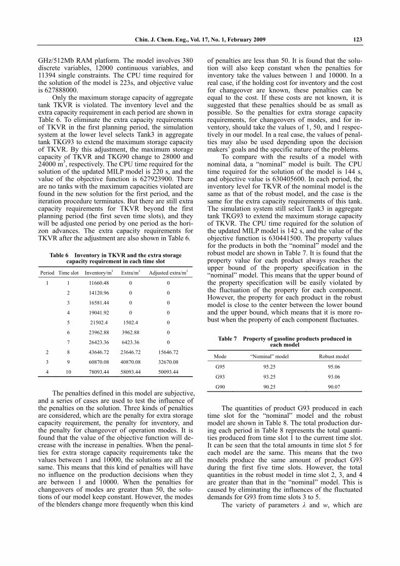
Only the maximum storage capacity of aggregate tank TKVR is violated. The inventory level and the extra capacity requirement in each period are shown in Table 6. To eliminate the extra capacity requirements of TKVR in the first planning period, the simulation system at the lower level selects Tank3 in aggregate tank TKG93 to extend the maximum storage capacity of TKVR. By this adjustment, the maximum storage capacity of TKVR and TKG90 change to 28000 and 24000 m3, respectively. The CPU time required for the solution of the updated MILP model is 220 s, and the value of the objective function is 627923900. There are no tanks with the maximum capacities violated are found in the new solution for the first period, and the iteration procedure terminates. But there are still extra capacity requirements for TKVR beyond the first planning period (the first seven time slots), and they will be adjusted one period by one period as the hori-zon advances. The extra capacity requirements for TKVR after the adjustment are also shown in Table 6.

Table 6 Inventory in TKVR and the extra storage capacity requirement in each time slot

Period Time slot Inventory/m3 Extra/m3 Adjusted extra/m3

1 1 11660.48 0 0

2 14120.96 0 0

3 16581.44 0 0

4 19041.92 0 0

5 21502.4 1502.4 0

6 23962.88 3962.88 0

7 26423.36 6423.36 0

2 8 43646.72 23646.72 15646.72

3 9 60870.08 40870.08 32670.08

4 10 78093.44 58093.44 50093.44

The penalties defined in this model are subjective, and a series of cases are used to test the influence of the penalties on the solution. Three kinds of penalties are considered, which are the penalty for extra storage capacity requirement, the penalty for inventory, and the penalty for changeover of operation modes. It is found that the value of the objective function will de-crease with the increase in penalties. When the penal-ties for extra storage capacity requirements take the values between 1 and 10000, the solutions are all the same. This means that this kind of penalties will have no influence on the production decisions when they are between 1 and 10000. When the penalties for changeovers of modes are greater than 50, the solu-tions of our model keep constant. However, the modes of the blenders change more frequently when this kind

of penalties are less than 50. It is found that the solu-tion will also keep constant when the penalties for inventory take the values between 1 and 10000. In a real case, if the holding cost for inventory and the cost for changeover are known, these penalties can be equal to the cost. If these costs are not known, it is suggested that these penalties should be as small as possible. So the penalties for extra storage capacity requirements, for changeovers of modes, and for in-ventory, should take the values of 1, 50, and 1 respec-tively in our model. In a real case, the values of penal-ties may also be used depending upon the decision makers’ goals and the specific nature of the problems.

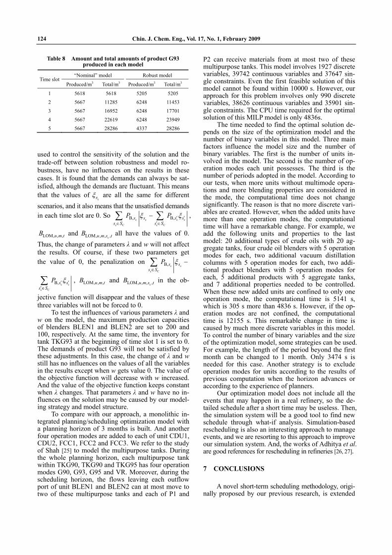
To compare with the results of a model with nominal data, a “nominal” model is built. The CPU time required for the solution of the model is 144 s, and objective value is 630405600. In each period, the inventory level for TKVR of the nominal model is the same as that of the robust model, and the case is the same for the extra capacity requirements of this tank. The simulation system still select Tank3 in aggregate tank TKG93 to extend the maximum storage capacity of TKVR. The CPU time required for the solution of the updated MILP model is 142 s, and the value of the objective function is 630441500. The property values for the products in both the “nominal” model and the robust model are shown in Table 7. It is found that the property value for each product always reaches the upper bound of the property specification in the “nominal” model. This means that the upper bound of the property specification will be easily violated by the fluctuation of the property for each component. However, the property for each product in the robust model is close to the center between the lower bound and the upper bound, which means that it is more ro-bust when the property of each component fluctuates.

Table 7 Property of gasoline products produced in each model

Mode “Nominal” model Robust model

G95 95.25 95.06

G93 93.25 93.06

G90 90.25 90.07

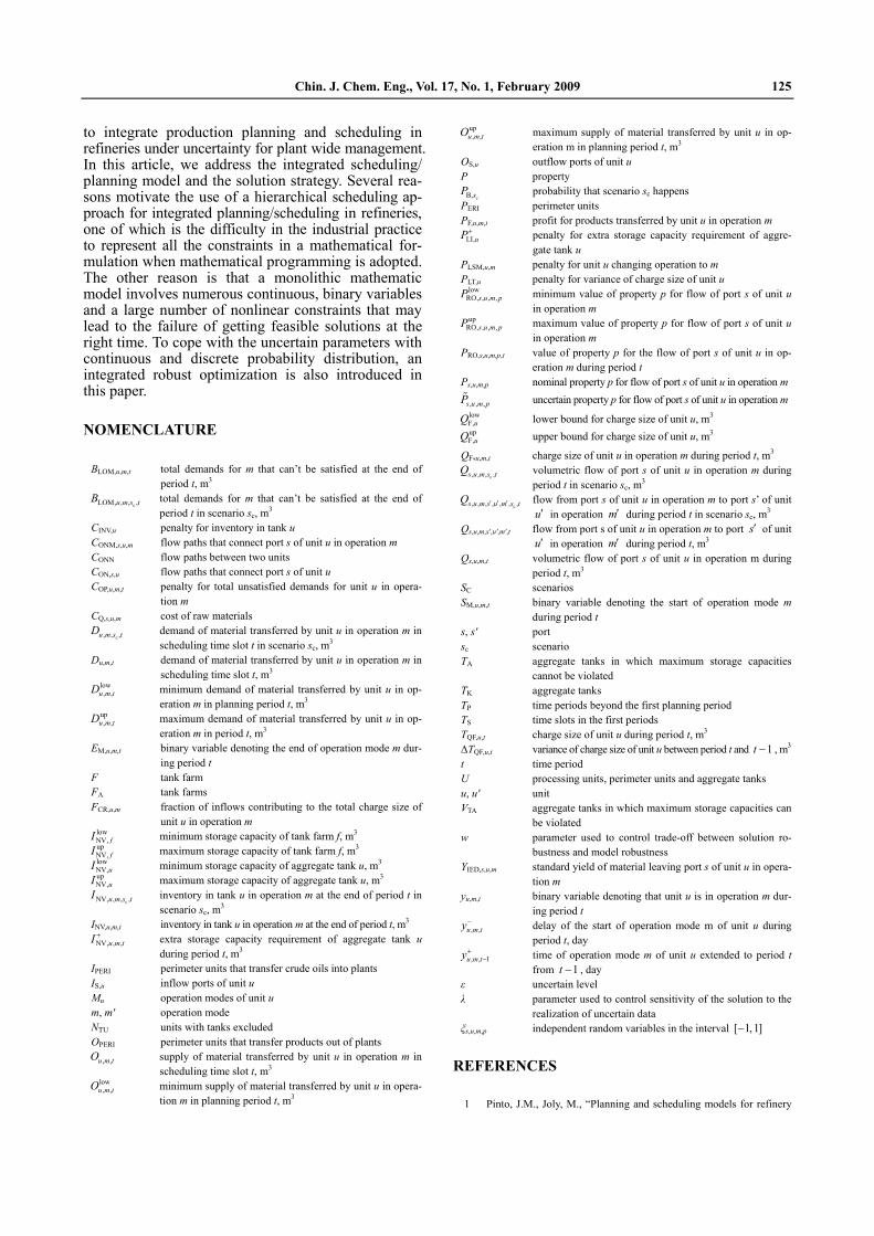
The quantities of product G93 produced in each time slot for the “nominal” model and the robust model are shown in Table 8. The total production dur-ing each period in Table 8 represents the total quanti-ties produced from time slot 1 to the current time slot. It can be seen that the total amounts in time slot 5 for each model are the same. This means that the two models produce the same amount of product G93 during the first five time slots. However, the total quantities in the robust model in time slot 2, 3, and 4 are greater than that in the “nominal” model. This is caused by eliminating the influences of the fluctuated demands for G93 from time slots 3 to 5.

The variety of parameters and w, which are


used to control the sensitivity of the solution and the trade-off between solution robustness and model ro-bustness, have no influences on the results in these cases. It is found that the demands can always be sat-isfied, although the demands are fluctuant. This means that the values of

cs are all the same for different scenarios, and it also means that the unsatisfied demands in each time slot are 0. So

c c c c

c C c C

B, B,s s s ss S s S

P P ,

LOM, , ,u m tB and cLOM, , , ,u m s tB all have the values of 0.

Thus, the change of parameters and w will not affect the results. Of course, if these two parameters get the value of 0, the penalization on

c c

c C

B,s ss S

P

c c

c C

B,s ss S

P , LOM, , ,u m tB and cLOM, , , ,u m s tB in the ob-

jective function will disappear and the values of these three variables will not be forced to 0.

To test the influences of various parameters and w on the model, the maximum production capacities of blenders BLEN1 and BLEN2 are set to 200 and 100, respectively. At the same time, the inventory for tank TKG93 at the beginning of time slot 1 is set to 0. The demands of product G93 will not be satisfied by these adjustments. In this case, the change of and w still has no influences on the values of all the variables in the results except when w gets value 0. The value of the objective function will decrease with w increased. And the value of the objective function keeps constant when changes. That parameters and w have no in-fluences on the solution may be caused by our model-ing strategy and model structure.

To compare with our approach, a monolithic in-tegrated planning/scheduling optimization model with a planning horizon of 3 months is built. And another four operation modes are added to each of unit CDU1, CDU2, FCC1, FCC2 and FCC3. We refer to the study of Shah [25] to model the multipurpose tanks. During the whole planning horizon, each multipurpose tank within TKG90, TKG90 and TKG95 has four operation modes G90, G93, G95 and VR. Moreover, during the scheduling horizon, the flows leaving each outflow port of unit BLEN1 and BLEN2 can at most move to two of these multipurpose tanks and each of P1 and

P2 can receive materials from at most two of these multipurpose tanks. This model involves 1927 discrete variables, 39742 continuous variables and 37647 sin-gle constraints. Even the first feasible solution of this model cannot be found within 10000 s. However, our approach for this problem involves only 990 discrete variables, 38626 continuous variables and 35901 sin-gle constraints. The CPU time required for the optimal solution of this MILP model is only 4836s.

The time needed to find the optimal solution de-pends on the size of the optimization model and the number of binary variables in this model. Three main factors influence the model size and the number of binary variables. The first is the number of units in-volved in the model. The second is the number of op-eration modes each unit possesses. The third is the number of periods adopted in the model. According to our tests, when more units without multimode opera-tions and more blending properties are considered in the mode, the computational time does not change significantly. The reason is that no more discrete vari-ables are created. However, when the added units have more than one operation modes, the computational time will have a remarkable change. For example, we add the following units and properties to the last model: 20 additional types of crude oils with 20 ag-gregate tanks, four crude oil blenders with 5 operation modes for each, two additional vacuum distillation columns with 5 operation modes for each, two addi-tional product blenders with 5 operation modes for each, 5 additional products with 5 aggregate tanks, and 7 additional properties needed to be controlled. When these new added units are confined to only one operation mode, the computational time is 5141 s, which is 305 s more than 4836 s. However, if the op-eration modes are not confined, the computational time is 12155 s. This remarkable change in time is caused by much more discrete variables in this model. To control the number of binary variables and the size of the optimization model, some strategies can be used. For example, the length of the period beyond the first month can be changed to 1 month. Only 3474 s is needed for this case. Another strategy is to exclude operation modes for units according to the results of previous computation when the horizon advances or according to the experience of planners.

Our optimization model does not include all the events that may happen in a real refinery, so the de-tailed schedule after a short time may be useless. Then, the simulation system will be a good tool to find new schedule through what-if analysis. Simulation-based rescheduling is also an interesting approach to manage events, and we are resorting to this approach to improve our simulation system. And, the works of Adhitya et al. are good references for rescheduling in refineries [26, 27].

7 CONCLUSIONS

A novel short-term scheduling methodology, origi-nally proposed by our previous research, is extended

Table 8 Amount and total amounts of product G93produced in each model

“Nominal” model Robust model Time slot

Produced/m3 Total/m3 Produced/m3 Total/m3

1 5618 5618 5205 5205

2 5667 11285 6248 11453

3 5667 16952 6248 17701

4 5667 22619 6248 23949

5 5667 28286 4337 28286


to integrate production planning and scheduling in refineries under uncertainty for plant wide management. In this article, we address the integrated scheduling/ planning model and the solution strategy. Several rea-sons motivate the use of a hierarchical scheduling ap-proach for integrated planning/scheduling in refineries, one of which is the difficulty in the industrial practice to represent all the constraints in a mathematical for-mulation when mathematical programming is adopted. The other reason is that a monolithic mathematic model involves numerous continuous, binary variables and a large number of nonlinear constraints that may lead to the failure of getting feasible solutions at the right time. To cope with the uncertain parameters with continuous and discrete probability distribution, an integrated robust optimization is also introduced in this paper.

NOMENCLATURE

BLOM,u,m,t total demands for m that can’t be satisfied at the end of period t, m3

cLOM, , , ,u m s tB total demands for m that can’t be satisfied at the end of period t in scenario sc, m3

CINV,u penalty for inventory in tank u CONM,s,u,m flow paths that connect port s of unit u in operation m CONN flow paths between two units CON,s,u flow paths that connect port s of unit u COP,u,m,t penalty for total unsatisfied demands for unit u in opera-

tion m CQ,s,u,m cost of raw materials

c, , ,u m s tD demand of material transferred by unit u in operation m in scheduling time slot t in scenario sc, m3

Du,m,t demand of material transferred by unit u in operation m in scheduling time slot t, m3

low, ,u m tD minimum demand of material transferred by unit u in op-

eration m in planning period t, m3 up, ,u m tD maximum demand of material transferred by unit u in op-

eration m in period t, m3 EM,u,m,t binary variable denoting the end of operation mode m dur-

ing period t F tank farm FA tank farms FCR,u,m fraction of inflows contributing to the total charge size of

unit u in operation m lowNV, fI minimum storage capacity of tank farm f, m3 upNV, fI maximum storage capacity of tank farm f, m3 lowNV,uI minimum storage capacity of aggregate tank u, m3 upNV,uI maximum storage capacity of aggregate tank u, m3

cNV, , , ,u m s tI inventory in tank u in operation m at the end of period t in scenario sc, m3

INV,u,m,t inventory in tank u in operation m at the end of period t, m3 NV, , ,u m tI extra storage capacity requirement of aggregate tank u

during period t, m3 IPERI perimeter units that transfer crude oils into plants IS,u inflow ports of unit u Mu operation modes of unit u m, m operation mode NTU units with tanks excluded OPERI perimeter units that transfer products out of plants

, ,u m tO supply of material transferred by unit u in operation m in scheduling time slot t, m3

low, ,u m tO minimum supply of material transferred by unit u in opera-

tion m in planning period t, m3

up, ,u m tO maximum supply of material transferred by unit u in op-

eration m in planning period t, m3 OS,u outflow ports of unit u P property

cB,sP probability that scenario sc happens PERI perimeter units PF,u,m,t profit for products transferred by unit u in operation m

LI,uP penalty for extra storage capacity requirement of aggre-gate tank u

PLSM,u,m penalty for unit u changing operation to m PLT,u penalty for variance of charge size of unit u

lowRO, , , ,s u m pP minimum value of property p for flow of port s of unit u

in operation m up

RO, , , ,s u m pP maximum value of property p for flow of port s of unit u in operation m

PRO,s,u,m,p,t value of property p for the flow of port s of unit u in op-eration m during period t

Ps,u,m,p nominal property p for flow of port s of unit u in operation m

, , ,s u m pP uncertain property p for flow of port s of unit u in operation m lowF,uQ lower bound for charge size of unit u, m3 upF,uQ upper bound for charge size of unit u, m3

QF,u,m,t charge size of unit u in operation m during period t, m3

c, , , ,s u m s tQ volumetric flow of port s of unit u in operation m during period t in scenario sc, m3

c, , , , , , ,s u m s u m s tQ flow from port s of unit u in operation m to port s’ of unit u in operation m during period t in scenario sc, m3

Qs,u,m,s ,u ,m ,t flow from port s of unit u in operation m to port s of unit u in operation m during period t, m3

Qs,u,m,t volumetric flow of port s of unit u in operation m during period t, m3

SC scenarios SM,u,m,t binary variable denoting the start of operation mode m

during period t s, s port sc scenario TA aggregate tanks in which maximum storage capacities

cannot be violated TK aggregate tanks TP time periods beyond the first planning period TS time slots in the first periods TQF,u,t charge size of unit u during period t, m3

TQF,u,t variance of charge size of unit u between period t and 1t , m3 t time period U processing units, perimeter units and aggregate tanks u, u unit VTA aggregate tanks in which maximum storage capacities can

be violated w parameter used to control trade-off between solution ro-

bustness and model robustness YIED,s,u,m standard yield of material leaving port s of unit u in opera-

tion m yu,m,t binary variable denoting that unit u is in operation m dur-

ing period t , ,u m ty delay of the start of operation mode m of unit u during

period t, day , , 1u m ty time of operation mode m of unit u extended to period t

from 1t , day uncertain level parameter used to control sensitivity of the solution to the

realization of uncertain data s,u,m,p independent random variables in the interval [ 1,1]

REFERENCES

1 Pinto, J.M., Joly, M., “Planning and scheduling models for refinery


operations”, Comput. Chem. Eng., 24, 2259 2276 (2000). 2 Jia, Z., Ierapetritou, M., “Efficient short-term scheduling of refinery

operations based on a continuous time formulation”, Comput. Chem. Eng., 28, 1001 1019 (2004).

3 Reddy, P.C.P., Karimi, I.A., “A new continuous-time formulation for scheduling crude oil operations”, Chem. Eng. Sci., 59, 1325 1341 (2004).

4 GÖthe-Lundgren, M., Lundgren, J.T., “An optimization model for refinery production scheduling”, Int. J. Prod. Econ., 78, 255 270 (2002).

5 Glismann, K., Gruhn, G., “Short-term scheduling and recipe optimi-zation of blending processes”, Comput. Chem. Eng., 25, 627 634 (2001).

6 Jia, Z., Ierapetritou, M., Kelly, J.D., “Refinery short-term scheduling using continuous time formulation: Crude-oil operations”, Ind. Eng. Chem. Res., 42, 3085 3097 (2003).

7 Moro, L.F.L., Pinto, J.M., “Mixed-integer programming approach for short-term crude oil scheduling”, Ind. Eng. Chem. Res., 43, 85 94 (2004).

8 Bhattacharya, S., Bose, S.K., “Mathematical model for scheduling operationsin cascaded continuous processing units”, Eur. J. Oper. Res., 182, 1 14 (2007).

9 Pinto, J.M., Joly, M., “Planning and scheduling models for refinery operations”, Comput. Chem. Eng., 24, 2259 (2000).

10 Floudas, C.A., Lin, X., “Continuous-time versus discrete-time ap-proaches for scheduling of chemical processes: A review”, Comput. Chem. Eng., 28, 2109 2129 (2004).

11 Paolucci, M., Sacile, R., “Allocating crude oil supply to port and re-finery tanks: A simulation-based decision support system”, Decision Support Syst., 33, 39 54 (2002).

12 Chryssolouris, G., Papakostas, N., “Refinery short-term scheduling with tank farm, inventory and distillation management: An inte-grated simulation-based approach”, Eur. J. Oper. Res., 166, 812 827 (2005).

13 Zhao, X.Q., RONG, G., “Blending scheduling under uncertainty based on particle swarm optimization algorithm”, Chin. J. Chem. Eng., 13, 535 541 (2005).

14 Van den Heever, S.A., Grossmann, I.E., “A strategy for the integra-tion of production planning and reactive scheduling in the optimiza-tion of a hydrogen supply network”, Comput. Chem. Eng., 27, 1813 1839 (2003).

15 Bassett, M.H., Dave, P., Doyle, F.J., Kudva, G.K., Pekny, J.F., Rek-laitis, G.V., Subramanyam, S., Miller, D.L., Zentner, M.G., “Perspec-tives on model based integration of process operations”, Comput. Chem. Eng., 20, 821 844 (1996).

16 Birewar, D.B., Grossmann, I.E., “Simultaneous production planning and scheduling of multiproduct batch plants”, Ind. Eng. Chem. Res., 29, 570 (1990).

17 Guill n, G., Badell, M., Espuna, A., Puigjaner, L., “Simultaneous optimization of process operations and financial decisions to en-hance the integrated planning/scheduling of chemical supply chains”, Comput. Chem. Eng., 30, 421 436 (2006).

18 Cheng, L.F., Subrahmanian, E., Westerberg, A.W., “A comparison of optimal control and stochastic programming from a formulation and computation perspective”, Comput. Chem. Eng., 29, 149 164 (2004).

19 Sahinidis, N.V., “Optimization under uncertainty: State-of-the-art and opportunities”, Comput. Chem. Eng., 28, 971 983 (2004).

20 Janak, S.L., Lin, X., Floudas, C.A., “A new robust optimization ap-proach for scheduling under uncertainty II. Uncertainty with known probability distribution”, Comput. Chem. Eng., 31, 171 195 (2007).

21 Leung, S.C.H., Tsang, S.O.S., Ng, W.L., Wu, Y., “A robust optimiza-tion model for multi-site production planning problem in an uncer-tain environment”, Eur. J. Oper. Res., 181, 224 238 (2007).

22 Luo, C.P., Rong, G., “Hierarchical approach for short-term schedul-ing in refineries”, Ind. Eng. Chem. Res., 46, 3656 3668 (2007).

23 Kelly, J.D., “Production modeling for multimodal operations”, Chemical Engineering Progress, 100, 44 47 (2004).

24 Kelly, J.D., “Logistics: The missing link in blend scheduling opti-mization”, Hydrocarbon Processing, 45 55 (2006).

25 Shah, N., “Mathematical programming techniques for crude oil scheduling”, Comput. Chem. Eng., 20, 1227 1232 (1996).

26 Adhitya, A., Srinivasan, R., Karimi, I.A., “A model-based resched-uling framework for managing abnormal supply chain events”, Comput. Chem. Eng., 31, 496 518 (2005).

27 Adhitya, A., Srinivasan, R., Karimi, I.A., “Heuristic rescheduling of crude oil operations to manage abnormal supply chain events”, AIChE J., 53, 397 422 (2007).

Appendix A: Other constraints in the planning/ scheduling model

Mass balance at each port:

ONM , , ,

, , , , , , , , ,( , , )

S S,, , ,s u m

s u m t s u m s u m ts u m C

u u

Q Q

u U t T s I m M (A-1)

ONM , , ,

, , , , , , , , ,( , , )

S S,, , ,s u m

s u m t s u m s u m ts u m C

u u

Q Q

u U t T s O m M (A-2)

Equality A-1 relates the volumetric flow of inflow port s with every flow that enters that port. Equality A-2 relates the volu-metric flow of each outflow port s with every flow that leaves that port. , , , , , ,s u m s u m tQ represents the flow leaving port s of unit u in operation mode m and entering port s of unit u in operation mode m during time slot t. , , ,s u m tQ represents the flow of port s of unit u in operation mode m during time slot t.

Capacity constraint for each unit (tanks excluded):

F, , , CR, , , , ,

TU S, ,u

u m t u m s u m ts IS

u

Q F Q

u N t T m M (A-3)

low up, , F, F, , , , , F,

TU S, ,u m t u u m t u m t u

u

y Q Q y Qu N m M t T (A-4)

, , TU S1 ,u

u m tm M

y u N T T (A-5)

The inflow ports of each unit in the model may not represent all the inflow ports of that unit in a real case, and A-3 relates the charge size of unit u with the total flows of the inflow ports. QF,u,m,t is the charge size of unit u in operation m during period t, and FCR,u,m is a parameter between 0 and 1 that specifies the fraction of the total flows contributing to the charge size of unit u in operation m. Constraint (A-4) specifies that the minimum and maximum volumetric capacity must be satisfied if unit u operates in mode m during time slot t. If unit u does not operate in mode m during time slot t (yu,m,t 0), the charge size of the unit in mode m during time slot t will be zero. Constraint A-5 specifies that these units can at most be in one operation mode during time slot t and may be idle during time slot t.

Variety of the charge size of each unit (tanks excluded):

QF, , F, , , TU S,u

u t u m tm M

T Q u N t T (A-6)

QF, , QF, , 1 QF, , TU S,u t u t u tT T T u N t T (A-7)

QF, , 1 QF, , QF, , TU S,u t u t u tT T T u N t T (A-8)

Equality A-6 calculates the charge size of unit u during time slot t. QF, ,u tT is the difference of the charge size between two adjacent time slots. Constraints A-7 and A-8 are used to avoid the negative value of QF, ,u tT because the objective function is to minimize the value of QF, ,u tT . the value of QF, ,u tT can become either ( QF, , QF, , 1u t u tT T ) or ( QF, , 1 QF, ,u t u tT T ) de-pending on which is positive.

Volume of each outflow port in one operation mode of a


unit (tanks excluded):

, , , F, , , IED, , ,

S, TU S, , ,s u m t u m t s u m

u u

Q Q Ys O u N m M t T (A-9)

Yield expressions in our approach are based on a standard value YIED,s,u,m, which is determined over average values ob-tained from plant data. In different modes of a processing unit, the materials produced have different yields.

Material balance equation for each tank (products with uncertain demands excluded):

NV, , , NV, , , 1 , , , , , ,

K S, S, S, , ,u m t u m t s u m t s u m t

u u

I I Q Qu T s I s O t T (A-10)

The inventory in each tank at the end of time slot t is equal to the inventory at the end of time slot 1t plus the amount of the flows entering the unit during time slot t minus the amount of flows leaving the unit during time slot t. The tanks used in this model are aggregate tanks. Each aggregate tank has only one operation mode, one inflow port, and one outflow port. The storage capacity of each aggregate tank can change by adjust-ing the operation mode of the multipurpose tanks included in it.

Changeover between operation modes:

, , 1 , , M, , ,

TU S, ( , ) , ,u m t u m t u m t

u

y y Eu N m m M t T m m (A-11)

, , , , 1 M, , ,

TU S, ,u m t u m t u m t

u

y y Su N m M t T (A-12)

Whenever there is an end of the operation mode m, constraint (A-11) forces the corresponding variable EM,u,m,t to take the

value 1. And whenever there is a start of the operation mode, constraint A-12 forces the corresponding variable SM,u,m,t to be 1.

Variable length of the operation modes: low

, , , , 1 , , F, F, , ,

up, , , , 1 , , F,

TU S, ,

u m t u m t u m t u u m t

u m t u m t u m t u

u

y y y Q Q

y y y Q

u N m M t T (A-13)

, , 1 M, , , S, ,u m t u m t u uy E u U m M t T (A-14)

, , M, , , TU S, ,u m t u m t uy S u N m M t T (A-15)

, , 1 , , TU S,u u

u m t u m tm M m M

y y u N t T (A-16)

The model in the first planning period is based on discrete time formulation with each time slot being 1 day, and this means that each operation mode can only start at the beginning of one day and end at the end of one day. To extend the model and allow the start and end of each operation mode at any point in a time slot, we use the methods mentioned by GÖthe-Lundgren and Lundgren [4]. The term , , 1u m ty means that operation mode m of unit u is extended from time slot 1t to t, and , ,u m ty represents the delay of the start of an operation mode m of unit u. Constraint (A-14) specifies that operation mode m can be extended to the next time slot only if there is an end of opera-tion mode in the next time slot. Constraint (A-15) ensures that operation mode m can be delayed only if this mode is started during time slot t. Constraint (A-16) ensures that the extended time equals the delayed time.

a strategy for the integration of production planning and scheduling in refineries under uncertainty

Documents