Repeatability and ReproducibilityCopyright 1999 by Engineered Software, Inc.

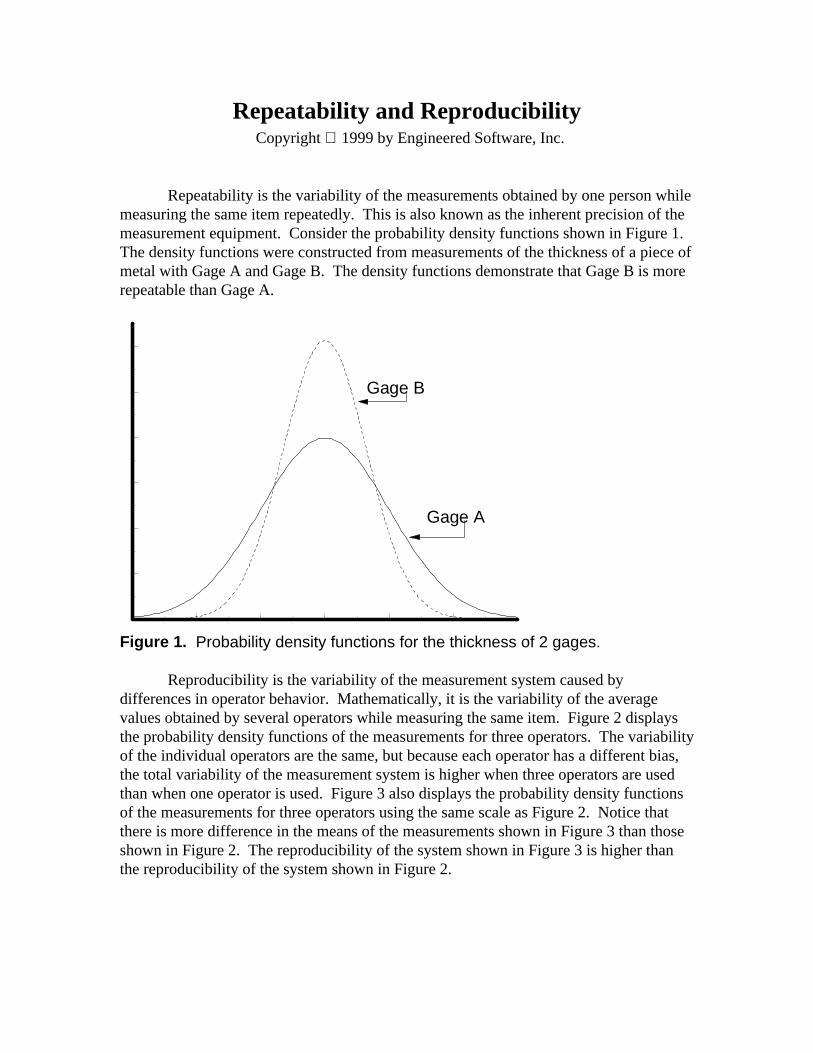
Repeatability is the variability of the measurements obtained by one person whilemeasuring the same item repeatedly. This is also known as the inherent precision of themeasurement equipment. Consider the probability density functions shown in Figure 1.The density functions were constructed from measurements of the thickness of a piece ofmetal with Gage A and Gage B. The density functions demonstrate that Gage B is morerepeatable than Gage A.

Gage A

Gage B

Figure 1. Probability density functions for the thickness of 2 gages.

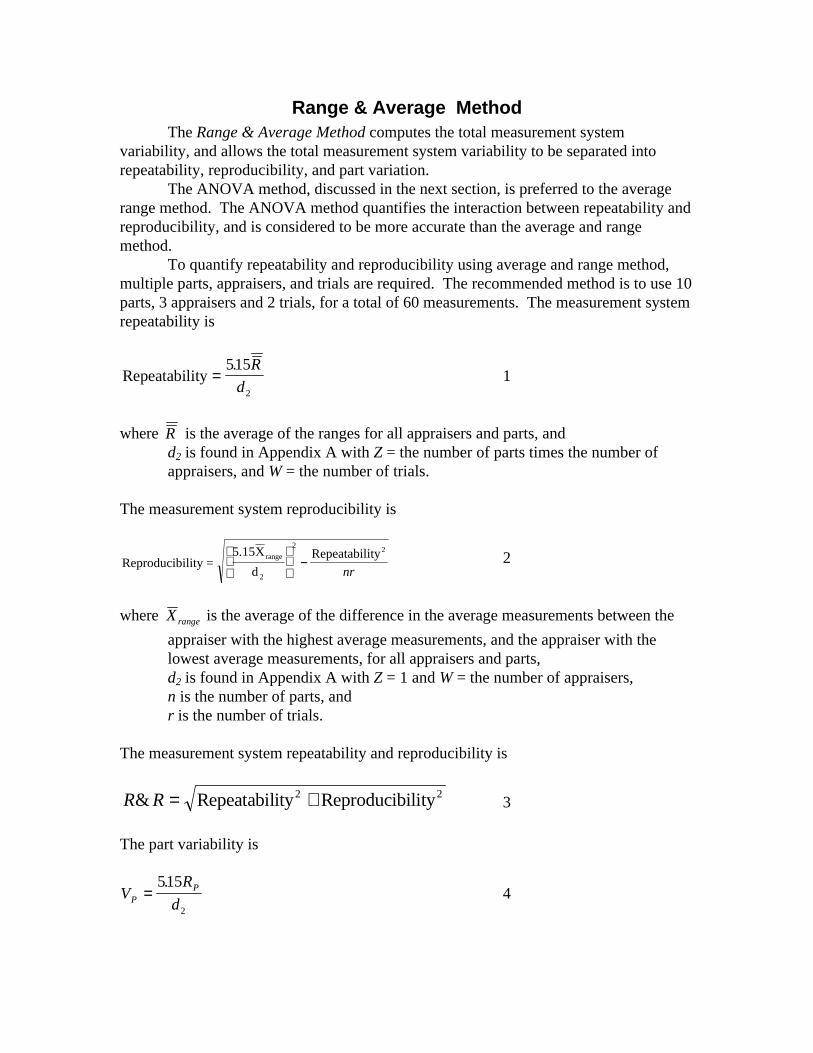
Reproducibility is the variability of the measurement system caused bydifferences in operator behavior. Mathematically, it is the variability of the averagevalues obtained by several operators while measuring the same item. Figure 2 displaysthe probability density functions of the measurements for three operators. The variabilityof the individual operators are the same, but because each operator has a different bias,the total variability of the measurement system is higher when three operators are usedthan when one operator is used. Figure 3 also displays the probability density functionsof the measurements for three operators using the same scale as Figure 2. Notice thatthere is more difference in the means of the measurements shown in Figure 3 than thoseshown in Figure 2. The reproducibility of the system shown in Figure 3 is higher thanthe reproducibility of the system shown in Figure 2.

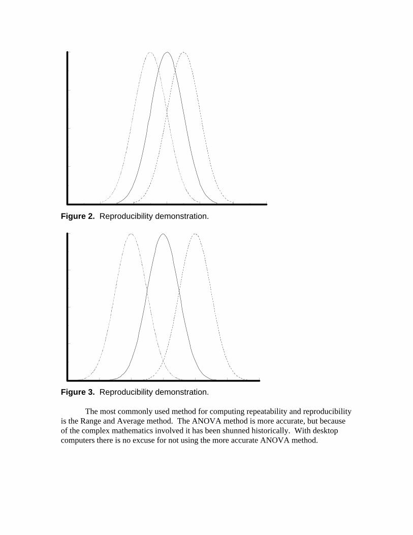
Figure 2. Reproducibility demonstration.

Figure 3. Reproducibility demonstration.

The most commonly used method for computing repeatability and reproducibilityis the Range and Average method. The ANOVA method is more accurate, but becauseof the complex mathematics involved it has been shunned historically. With desktopcomputers there is no excuse for not using the more accurate ANOVA method.

Range & Average MethodThe Range & Average Method computes the total measurement system

variability, and allows the total measurement system variability to be separated intorepeatability, reproducibility, and part variation.

The ANOVA method, discussed in the next section, is preferred to the averagerange method. The ANOVA method quantifies the interaction between repeatability andreproducibility, and is considered to be more accurate than the average and rangemethod.

To quantify repeatability and reproducibility using average and range method,multiple parts, appraisers, and trials are required. The recommended method is to use 10parts, 3 appraisers and 2 trials, for a total of 60 measurements. The measurement systemrepeatability is

Repeatability=515

2

. R

d1

where R is the average of the ranges for all appraisers and parts, andd2 is found in Appendix A with Z = the number of parts times the number ofappraisers, and W = the number of trials.

The measurement system reproducibility is

Reproducibility =5.15X

d

Repeatabilityrange

2

−

22

nr2

where Xrange is the average of the difference in the average measurements between the

appraiser with the highest average measurements, and the appraiser with thelowest average measurements, for all appraisers and parts,d2 is found in Appendix A with Z = 1 and W = the number of appraisers,n is the number of parts, andr is the number of trials.

The measurement system repeatability and reproducibility is

R R& = +Repeatability Reproducibility2 23

The part variability is

VR

dPP=

515

2

.4

where Rp is the difference between the largest average part measurement and the smallestaverage part measurement, where the average is taken for all appraisers and alltrials, andd2 is found in Appendix A with Z = 1 and W = the number of parts.

The total variability, measurement system variability and part variation combined is

V R R VT P= +& 2 2 5

Example 1The thickness, in millimeters, of 10 parts have been measured by 3 operators, using thesame measurement equipment. Each operator measured each part twice, and the data isgiven in Table 1.

Table 1. Range & Average method example data.Operator

A B CPart Trial 1 Trial 2 Trial 1 Trial 2 Trial 1 Trial 2

1 65.2 60.1 62.9 56.3 71.6 60.62 85.8 86.3 85.7 80.5 92.0 87.43 100.2 94.8 100.1 94.5 107.3 104.44 85.0 95.1 84.8 90.3 92.3 94.65 54.7 65.8 51.7 60.0 58.9 67.26 98.7 90.2 92.7 87.2 98.9 93.57 94.5 94.5 91.0 93.4 95.4 103.38 87.2 82.4 83.9 78.8 93.0 85.89 82.4 82.2 80.7 80.3 87.9 88.110 100.2 104.9 99.7 103.2 104.3 111.5

Repeatability is computed using the average of the ranges for all appraiser and allparts. This data is given in Table 2.

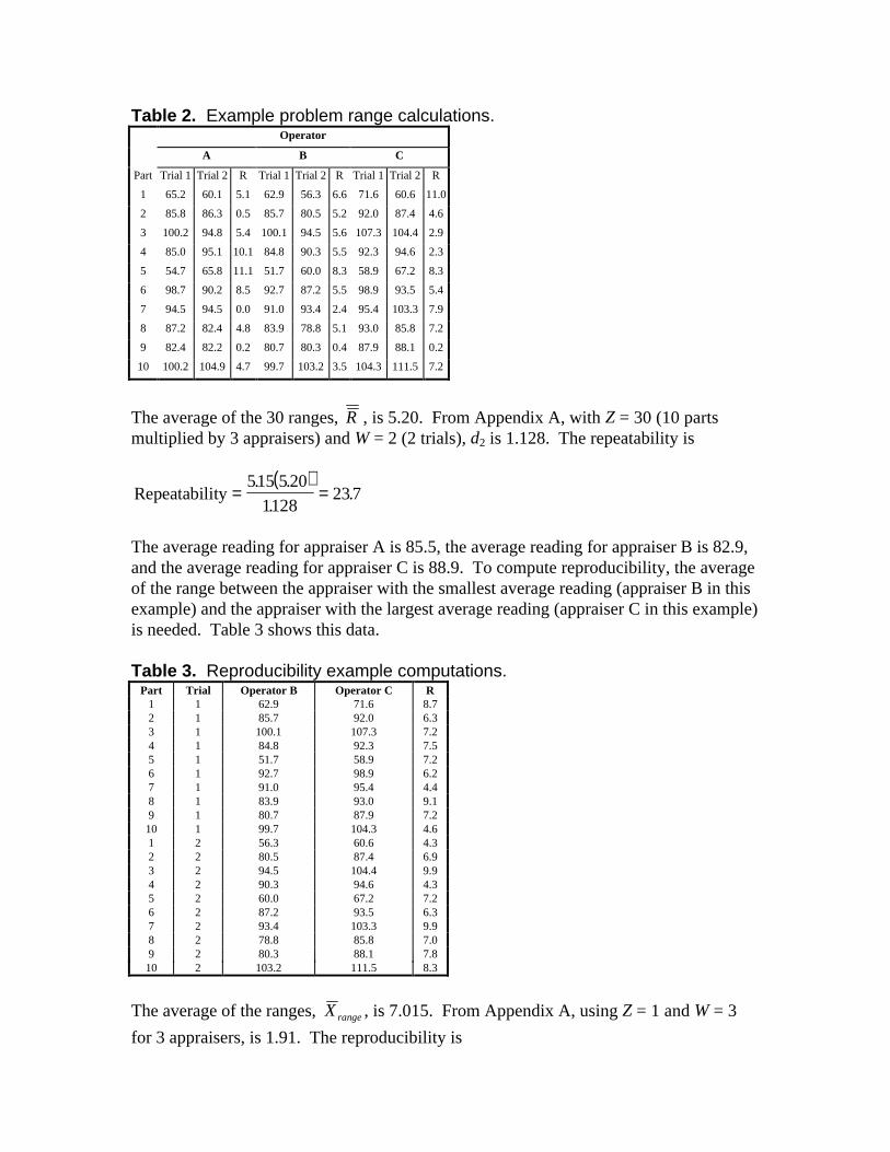
Table 2. Example problem range calculations.Operator

A B C

Part Trial 1 Trial 2 R Trial 1 Trial 2 R Trial 1 Trial 2 R

1 65.2 60.1 5.1 62.9 56.3 6.6 71.6 60.6 11.0

2 85.8 86.3 0.5 85.7 80.5 5.2 92.0 87.4 4.6

3 100.2 94.8 5.4 100.1 94.5 5.6 107.3 104.4 2.9

4 85.0 95.1 10.1 84.8 90.3 5.5 92.3 94.6 2.3

5 54.7 65.8 11.1 51.7 60.0 8.3 58.9 67.2 8.3

6 98.7 90.2 8.5 92.7 87.2 5.5 98.9 93.5 5.4

7 94.5 94.5 0.0 91.0 93.4 2.4 95.4 103.3 7.9

8 87.2 82.4 4.8 83.9 78.8 5.1 93.0 85.8 7.2

9 82.4 82.2 0.2 80.7 80.3 0.4 87.9 88.1 0.2

10 100.2 104.9 4.7 99.7 103.2 3.5 104.3 111.5 7.2

The average of the 30 ranges, R , is 5.20. From Appendix A, with Z = 30 (10 partsmultiplied by 3 appraisers) and W = 2 (2 trials), d2 is 1.128. The repeatability is

( )Repeatability= =

515 520

1128237

. .

..

The average reading for appraiser A is 85.5, the average reading for appraiser B is 82.9,and the average reading for appraiser C is 88.9. To compute reproducibility, the averageof the range between the appraiser with the smallest average reading (appraiser B in thisexample) and the appraiser with the largest average reading (appraiser C in this example)is needed. Table 3 shows this data.

Table 3. Reproducibility example computations.Part Trial Operator B Operator C R

1 1 62.9 71.6 8.72 1 85.7 92.0 6.33 1 100.1 107.3 7.24 1 84.8 92.3 7.55 1 51.7 58.9 7.26 1 92.7 98.9 6.27 1 91.0 95.4 4.48 1 83.9 93.0 9.19 1 80.7 87.9 7.210 1 99.7 104.3 4.61 2 56.3 60.6 4.32 2 80.5 87.4 6.93 2 94.5 104.4 9.94 2 90.3 94.6 4.35 2 60.0 67.2 7.26 2 87.2 93.5 6.37 2 93.4 103.3 9.98 2 78.8 85.8 7.09 2 80.3 88.1 7.810 2 103.2 111.5 8.3

The average of the ranges, Xrange, is 7.015. From Appendix A, using Z = 1 and W = 3

for 3 appraisers, is 1.91. The reproducibility is

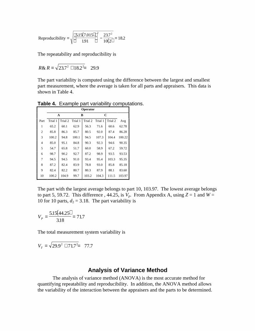
( )( )Reproducibility=

− =515 7 015

191

237

10 218 2

2 2. .

.

..

The repeatability and reproducibility is

R R& . . .= + =237 18 2 29 92 2

The part variability is computed using the difference between the largest and smallestpart measurement, where the average is taken for all parts and appraisers. This data isshown in Table 4.

Table 4. Example part variability computations.Operator

A B C

Part Trial 1 Trial 2 Trial 1 Trial 2 Trial 1 Trial 2 Avg

1 65.2 60.1 62.9 56.3 71.6 60.6 62.78

2 85.8 86.3 85.7 80.5 92.0 87.4 86.28

3 100.2 94.8 100.1 94.5 107.3 104.4 100.22

4 85.0 95.1 84.8 90.3 92.3 94.6 90.35

5 54.7 65.8 51.7 60.0 58.9 67.2 59.72

6 98.7 90.2 92.7 87.2 98.9 93.5 93.53

7 94.5 94.5 91.0 93.4 95.4 103.3 95.35

8 87.2 82.4 83.9 78.8 93.0 85.8 85.18

9 82.4 82.2 80.7 80.3 87.9 88.1 83.60

10 100.2 104.9 99.7 103.2 104.3 111.5 103.97

The part with the largest average belongs to part 10, 103.97. The lowest average belongsto part 5, 59.72. This difference , 44.25, is Vp. From Appendix A, using Z = 1 and W =10 for 10 parts, d2 = 3.18. The part variability is

( )VP = =

515 44 25

318717

. .

..

The total measurement system variability is

VT = + =29 9 717 77 72 2. . .

Analysis of Variance MethodThe analysis of variance method (ANOVA) is the most accurate method for

quantifying repeatability and reproducibility. In addition, the ANOVA method allowsthe variability of the interaction between the appraisers and the parts to be determined.

The ANOVA method for measurement assurance is the same statistical techniqueused to analyze the effects of different factors in designed experiments. The ANOVAdesign used is a two-way, fixed effects model with replications. The ANOVA table isshown in Table 5.

Table 5 . Two-Way ANOVA Table.Source ofVariation

Sum ofSquare

s

Degreesof

Freedom

MeanSquare F Statistic

Appraiser SSA a-1MSA

SSA

a=

−1F

MSA

MSE=

Parts SSB b-1MSB

SSB

b=

−1F

MSB

MSE=

Interaction(Appraiser,

Parts)

SSAB (a-1)(b-1) MSABSSAB

a b=

− −( )( )1 1 FM SA B

M SE=

Gage(Error)

SSE ab(n-1)MSE

SSE

ab n=

−( )1

Total TSS N-1

SSAY

bn

Y

Ni

i

a

= − ••

=∑ ( )..

2 2

1

6

SSBY

an

Y

Nj

j

b

= − ••

=∑

( ). .2 2

1

7

SSABY

n

Y

NSSA SSB

ij

j

b

i

a

= − − −••

==∑∑

( ).2 2

11

8

TSS YY

Nijkk

n

j

b

i

a

= − ••

===∑∑∑ 2

2

111

9

SSE TSS SSA SSB SSAB= − − − 10

a = number of appraisers,b = number parts,n = the number of trials, andN = total number of readings (abn)

When conducting a study, the recommended procedure is to use 10 parts, 3appraisers and 2 trials, for a total of 60 measurements. The measurement systemrepeatability is

Repeatability= 515. MSE 11

The measurement system reproducibility is

Reproducibility=−

515.MSA MSAB

bn12

The interaction between the appraisers and the parts is

I =−

515.MSAB MSE

n13

The measurement system repeatability and repeatability is

R R I& = + +Repeatability Reproducibility2 2 2 14

The measurement system part variation is

VMSB MSAB

anP =−

515. 15

The total measurement system variation is

V R R VT P= +& 2 2 16

Example 2The thickness, in millimeters, of 10 parts have been measured by 3 operators, using thesame measurement equipment. Each operator measured each part twice, and the data isgiven in Table 6.

Table 6. ANOVA method example data.Operator

A B C

Part Trial 1 Trial 2 Trial 1 Trial 2 Trial 1 Trial 2

1 65.2 60.1 62.9 56.3 71.6 60.6

2 85.8 86.3 85.7 80.5 92.0 87.4

3 100.2 94.8 100.1 94.5 107.3 104.4

4 85.0 95.1 84.8 90.3 92.3 94.6

5 54.7 65.8 51.7 60.0 58.9 67.2

6 98.7 90.2 92.7 87.2 98.9 93.5

7 94.5 94.5 91.0 93.4 95.4 103.3

8 87.2 82.4 83.9 78.8 93.0 85.8

9 82.4 82.2 80.7 80.3 87.9 88.1

10 100.2 104.9 99.7 103.2 104.3 111.5

To compute the characteristics of this measurement system, the two-wayANOVA table must be completed. The sum of the 20 readings (10 parts multiplied by 2trials) for appraiser A is 1710.2. The sum of the 20 readings for appraiser B is 1657.7.

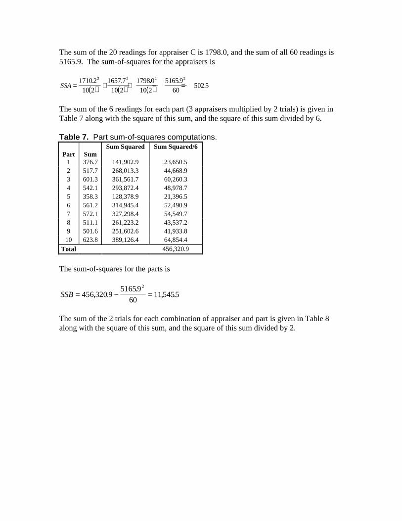
The sum of the 20 readings for appraiser C is 1798.0, and the sum of all 60 readings is5165.9. The sum-of-squares for the appraisers is

( ) ( ) ( )SSA= + + − =17102

10 2

1657 7

10 2

17980

10 2

51659

60502 5

2 2 2 2. . . ..

The sum of the 6 readings for each part (3 appraisers multiplied by 2 trials) is given inTable 7 along with the square of this sum, and the square of this sum divided by 6.

Table 7. Part sum-of-squares computations.

Part SumSum Squared Sum Squared/6

1 376.7 141,902.9 23,650.52 517.7 268,013.3 44,668.93 601.3 361,561.7 60,260.34 542.1 293,872.4 48,978.75 358.3 128,378.9 21,396.56 561.2 314,945.4 52,490.97 572.1 327,298.4 54,549.78 511.1 261,223.2 43,537.29 501.6 251,602.6 41,933.810 623.8 389,126.4 64,854.4

Total 456,320.9

The sum-of-squares for the parts is

SSB= − =456 320 951659

60115455

2

, ..

, .

The sum of the 2 trials for each combination of appraiser and part is given in Table 8along with the square of this sum, and the square of this sum divided by 2.

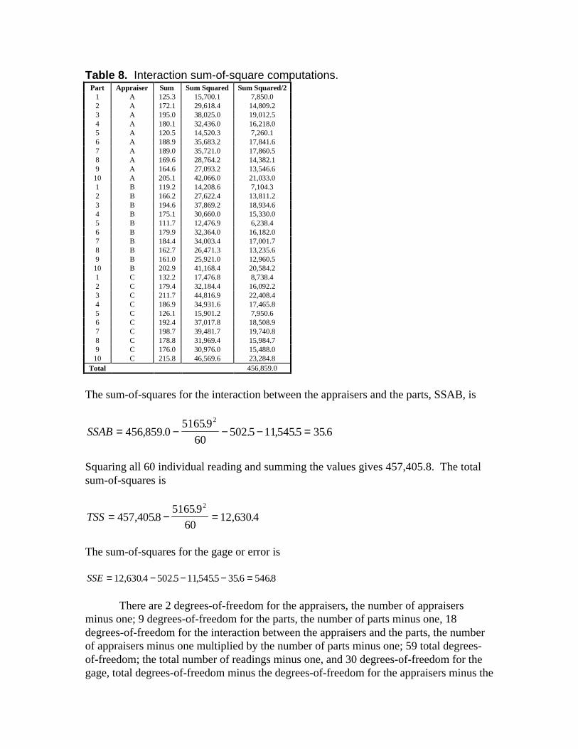
Table 8. Interaction sum-of-square computations.Part Appraiser Sum Sum Squared Sum Squared/2

1 A 125.3 15,700.1 7,850.02 A 172.1 29,618.4 14,809.23 A 195.0 38,025.0 19,012.54 A 180.1 32,436.0 16,218.05 A 120.5 14,520.3 7,260.16 A 188.9 35,683.2 17,841.67 A 189.0 35,721.0 17,860.58 A 169.6 28,764.2 14,382.19 A 164.6 27,093.2 13,546.610 A 205.1 42,066.0 21,033.01 B 119.2 14,208.6 7,104.32 B 166.2 27,622.4 13,811.23 B 194.6 37,869.2 18,934.64 B 175.1 30,660.0 15,330.05 B 111.7 12,476.9 6,238.46 B 179.9 32,364.0 16,182.07 B 184.4 34,003.4 17,001.78 B 162.7 26,471.3 13,235.69 B 161.0 25,921.0 12,960.510 B 202.9 41,168.4 20,584.21 C 132.2 17,476.8 8,738.42 C 179.4 32,184.4 16,092.23 C 211.7 44,816.9 22,408.44 C 186.9 34,931.6 17,465.85 C 126.1 15,901.2 7,950.66 C 192.4 37,017.8 18,508.97 C 198.7 39,481.7 19,740.88 C 178.8 31,969.4 15,984.79 C 176.0 30,976.0 15,488.010 C 215.8 46,569.6 23,284.8

Total 456,859.0

The sum-of-squares for the interaction between the appraisers and the parts, SSAB, is

SSAB= − − − =456 859 051659

60502 5 115455 356

2

, ..

. , . .

Squaring all 60 individual reading and summing the values gives 457,405.8. The totalsum-of-squares is

TSS= − =457 405851659

6012 630 4

2

, ..

, .

The sum-of-squares for the gage or error is

SSE= − − − =12 630 4 502 5 115455 356 5468, . . , . . .

There are 2 degrees-of-freedom for the appraisers, the number of appraisersminus one; 9 degrees-of-freedom for the parts, the number of parts minus one, 18degrees-of-freedom for the interaction between the appraisers and the parts, the numberof appraisers minus one multiplied by the number of parts minus one; 59 total degrees-of-freedom; the total number of readings minus one, and 30 degrees-of-freedom for thegage, total degrees-of-freedom minus the degrees-of-freedom for the appraisers minus the

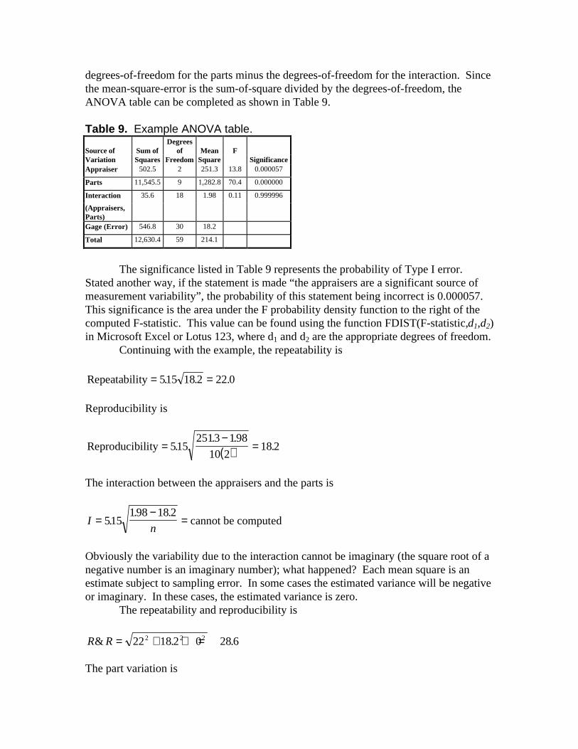
degrees-of-freedom for the parts minus the degrees-of-freedom for the interaction. Sincethe mean-square-error is the sum-of-square divided by the degrees-of-freedom, theANOVA table can be completed as shown in Table 9.

Table 9. Example ANOVA table.

Source of Sum ofDegrees

of Mean FVariation Squares Freedom Square SignificanceAppraiser 502.5 2 251.3 13.8 0.000057

Parts 11,545.5 9 1,282.8 70.4 0.000000

Interaction 35.6 18 1.98 0.11 0.999996

(Appraisers,Parts)Gage (Error) 546.8 30 18.2

Total 12,630.4 59 214.1

The significance listed in Table 9 represents the probability of Type I error.Stated another way, if the statement is made “the appraisers are a significant source ofmeasurement variability”, the probability of this statement being incorrect is 0.000057.This significance is the area under the F probability density function to the right of thecomputed F-statistic. This value can be found using the function FDIST(F-statistic,d1,d2)in Microsoft Excel or Lotus 123, where d1 and d2 are the appropriate degrees of freedom.

Continuing with the example, the repeatability is

Repeatability= =515 18 2 22 0. . .

Reproducibility is

( )Reproducibility=−

=5152513 198

10 218 2.

. ..

The interaction between the appraisers and the parts is

In

=−

=515198 18 2

.. .

cannot be computed

Obviously the variability due to the interaction cannot be imaginary (the square root of anegative number is an imaginary number); what happened? Each mean square is anestimate subject to sampling error. In some cases the estimated variance will be negativeor imaginary. In these cases, the estimated variance is zero.

The repeatability and reproducibility is

R R& . .= + + =22 18 2 0 28 62 2 2

The part variation is

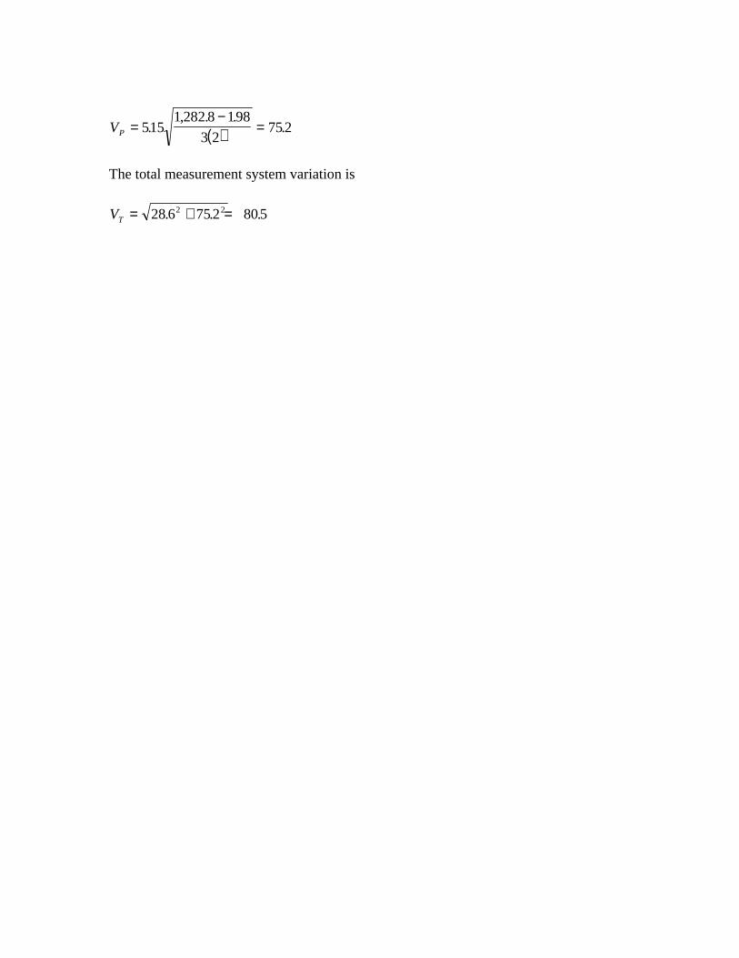
( )VP =−

=5151 282 8 198

3 2752.

, . ..

The total measurement system variation is

VT = + =28 6 752 8052 2. . .

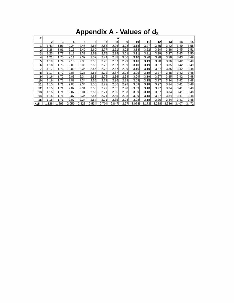
Appendix A - Values of d 2z w

2 3 4 5 6 7 8 9 10 11 12 13 14 151 1.41 1.91 2.24 2.48 2.67 2.83 2.96 3.08 3.18 3.27 3.35 3.42 3.49 3.552 1.28 1.81 2.15 2.40 2.60 2.77 2.91 3.02 3.13 3.22 3.30 3.38 3.45 3.513 1.23 1.77 2.12 2.38 2.58 2.75 2.89 3.01 3.11 3.21 3.29 3.37 3.43 3.504 1.21 1.75 2.11 2.37 2.57 2.74 2.88 3.00 3.10 3.20 3.28 3.36 3.43 3.495 1.19 1.74 2.10 2.36 2.56 2.78 2.87 2.99 3.10 3.19 3.28 3.36 3.42 3.496 1.18 1.73 2.09 2.35 2.56 2.73 2.87 2.99 3.10 3.19 3.27 3.35 3.42 3.497 1.17 1.73 2.09 2.35 2.55 2.72 2.87 2.99 3.10 3.19 3.27 3.35 3.42 3.488 1.17 1.72 2.08 2.35 2.55 2.72 2.87 2.98 3.09 3.19 3.27 3.35 3.42 3.489 1.16 1.72 2.08 2.34 2.55 2.72 2.86 2.98 3.09 3.19 3.27 3.35 3.42 3.48

10 1.16 1.72 2.08 2.34 2.55 2.72 2.86 2.98 3.09 3.18 3.27 3.34 3.42 3.4811 1.15 1.71 2.08 2.34 2.55 2.72 2.86 2.98 3.09 3.18 3.27 3.34 3.41 3.4812 1.15 1.71 2.07 2.34 2.55 2.72 2.85 2.98 3.09 3.18 3.27 3.34 3.41 3.4813 1.15 1.71 2.07 2.34 2.55 2.71 2.85 2.98 3.09 3.18 3.27 3.34 3.41 3.4814 1.15 1.71 2.07 2.34 2.54 2.71 2.85 2.98 3.09 3.18 3.27 3.34 3.41 3.4815 1.15 1.71 2.07 2.34 2.54 2.71 2.85 2.98 3.08 3.18 3.26 3.34 3.41 3.48

>15 1.128 1.693 2.059 2.326 2.534 2.704 2.847 2.97 3.078 3.173 3.258 3.336 3.407 3.472