Time Varying Market Integration as a regime switching process

Lakshmi Narasimhan SFellow of XLRI

XLRI, Jamshedpur, IndiaEmail: lakshmi.01@astra.xlri.ac.in

Phone: 0657-225506 Extn (254)

Dr H.K. PradhanProfessor of Finance & Economics

XLRI, Jamshedpur, India Email: pradhan@xlri.ac.in

Phone: 0657-225506 Extn (401)

Time Varying Market Integration as a regime switching process

Abstract

We attempt to estimate the likelihood of the integration of Indian stocks with the world

market using Markov regime switching model. Bekaert and Harvey (1995)’s empirical

model has been suitably extended to accommodate GARCH-M effect to estimate the level

of integration. Given the small sample size, the maximum likelihood estimates have been

estimated using an innovative grid approach. The level of integration clearly varies with

the size of the stocks: larger stocks are more integrated than smaller stocks. Time

varying integration plots are used to identify the change in the level of integration with

important events that took place in Indian/International capital markets.

1.1. Market Integration and Asset Pricing

Asset-pricing models assume a priori whether the capital markets are perfectly integrated

or segmented. Or in other words, asset-pricing models can be broadly classified into (1)

models that assume that the markets are integrated and (2) models that assume that the

markets are segmented. This assumption is very crucial as it affects the optimal portfolio

choice of investors in mean-variance framework. Stulz (1981a) defines market

integration as the condition where “ two assets which belong to different countries but

have the same risk with respect to some model of international asset pricing without

barriers to international investment should have same expected returns”. Otherwise it

would result in arbitrage situation.

However the term "without barriers to international investment" is note worthy because

existence of barriers in any form could prevent capital markets from being perfectly

integrated even when foreign portfolio investments are allowed. These barriers can take

the form of quantitative or qualitative restrictions. Differential tax rates, restrictions on

the ownership, different classes of assets are the very popular form of restrictions used by

the local governments to restrict foreign portfolio investments. The qualitative

restrictions arise because of asymmetric information between the domestic and foreign

investors, unfamiliarity with the domestic market functioning.

Asset pricing under perfect market integration: Studies that assume that markets are

perfectly integrated, in fact, assume that such barriers do not exist and test their asset

pricing models. The departures found from their hypotheses are considered evidence of

the existence of barriers. Harvey (1991), Dumas and Solnik (1995), Wheatley (1988),

Solnik (1983), Cho, Eun and Senbet (1986), Ferson and Harvey (1993, 1994a, 1994b),

Campbell and Hamao (1992), Bekaert and Hodrick (1992) and Harvey, Solnik and Zhou

(1994) are some of the very important under this category1.

Transaction barriers and Market Segmentation

The second group of studies that assumes that markets are segmented considers various

types of barriers explicitly in their models and test for their presence. Some of the

barriers that are considered are: Differential tax rates, Existence of different classes of

assets, quantitative restrictions on the ownership. In the presence of differential taxes for

domestic investors and foreign investors, global investors would have to optimize their

investments based on the after tax returns instead of pre tax returns. This idea was

incorporated by Black (1972). Many countries used to have different classes of securities

for foreign portfolio investors to differentiate them from the domestic investors and

fungibility was not allowed between these two classes of securities. This results in the

assets on which foreign investors trade being traded at a premium compared to the shares

traded by the domestic investors. Domowitz, Glenn and Madhavan (1997) estimate the

cost of ownership restrictions for Mexican market where multiple classes of equity shares

exist. Huge premiums that existed between the GDR/ADR issued by Indian companies

and the price of the corresponding underlying shares listed in Indian stock market when

two-way fungibility2 was not allowed is evidence to this phenomenon.

1 For detailed references on this please refer Harvey (1991).2 Two-way fungibility allows the conversion of ADR/GDRs into underlying shares and reconversion of the same into depository receipts. Before June'2002, only one way fungibility was allowed, i.e. ADR/GDRs can be converted into underlying shares and the reverse was not allowed. This barred the process of arbitrage and resulted in ADR/GDRs being traded at a huge premium compared to the price of underlying

Besides, local Governments can enforce restrictions on the maximum foreign ownership

allowed in any domestic firms thus preventing the foreign investors to hold their optimal

portfolio choices. For example, in India, no single foreign institutional investor can hold

more than 10% in any of the Indian companies and FIIs as a group cannot hold more than

25%. This can be increased up to 40% with the permission of the shareholders3. These

ownership restrictions are explicitly modelled in Eun and Janakiraman (1986) and Alford

(1990).

Given these barriers to foreign investments, Errunza and Losq (1985, 1989) take asset

pricing a step close to the reality where the capital markets are neither fully integrated nor

fully segmented. In their model of partial integration/segmentation, there are two types

of securities; eligible securities where the foreign investors can participate and the rest

are ineligible securities in which only domestic investors can invest. In this situation, the

eligible securities shall be priced as if the markets are perfectly integrated and the

ineligible securities are priced in the segmented market framework. However, an

important assumption in their model is that that the extent of integration/segmentation of

the capital market remains constant.

The qualitative barriers arise because the foreign investors would be unfamiliar with the

local market functioning and there could be asymmetric information between the local

and foreign investors or the cost of obtaining information is significant enough to give

different returns for foreign and domestic investors. This result in a situation termed as

‘home bias’ in the literature, where in portfolio of foreign investors is dominated by

assets from their respective domestic markets in spite of superior returns that can be

achieved through international diversification. In the section that follows we focus on

the studies that look into the integration of emerging markets.

1.2. Emerging markets and Time varying Market Integration

share listed in Indian stock market. 3 Even there are differences in voting rights also thus making the foreign investment funds to be just an investment agencies without any interest for ownership control.

Emerging markets provide a very good case for the testing of capital market integration

and its effects. Most of the emerging markets started liberalizing their capital markets

(including allowing foreign portfolio investment) from late eighties through early

nineties. However, the two main hurdles in empirical testing these propositions are (1)

dating the liberalization and (2) time varying integration of capital markets.

Authors who have studied the impact of liberalization on emerging markets have handled

this issue by using various mile stone events as a proxy for starting date of liberalization

viz., listing of first depository receipts, launching of first country fund, starting of foreign

portfolio investments etc (Henry, 2000a and 2000b, Bekaert and Harvey, 2000).

Alternatively, testing for structural breaks in the return generating process to see their

coincidence with any of the milestone events is done (Bekaert, Harvey and Lumsdaine,

2002)

The second hurdle arises because the capital market integration due to liberalization

measures is very smooth. Even after the domestic markets are opened up, foreign

investors would take some time to get acclimatized with the local market conditions. In

the case of Indian market, FIIs were allowed officially from Sept 1992 but the

investments started flowing in only after several months (Shah and Sivsankar, 2000).

Also reversion of liberalization policies by the respective Governments can also hamper

integration of markets. After the South East Asian crisis, the Thailand Government have

imposed new restrictions on foreign investments to strengthen their financial system.

Another pointer towards time varying market integration is the empirical finding that

capital markets become more integrated during highly volatile periods (or contagion

effect). The big market crash of 1987 in USA and its repercussion on various markets in

Europe and Asia is the best indication of the integration of capital markets.

Bekaert and Harvey (1995) address these empirical issues in their model for time varying

world market integration based on Hamilton's regime switching model. They show that

emerging markets4 indeed become more integrated with the world market over time. The

measure of integration/segmentation in their study is the probability/likelihood of the

capital market being in the integrated/segmented state. The ‘time varying integration’

issue is answered by allowing the likelihood of integration to vary over time. Since the

integration of the market is determined from the behavior of the ex post data, the issue of

dating of liberalization also do not arise. Our study, take Bekaert and Harvey (1995)

forward to test the integration at portfolio level. The following section discuss about the

empirical studies on Indian securities market where inferences can be drawn about the

market integration.

1.3. Indian Studies on market integration

Indian studies related to capital market integration can be classified into two types. The

first group of studies examines the stocks that are listed in multiple stock exchanges and

compare their returns. Under the perfectly integrated market condition the returns from

the stocks on these exchanges should mimic each other. Listing of depository receipts on

American and European stock exchanges provide an ideal opportunity to test this.

The second group of studies focuses on testing whether the factors that determine stock

market returns are the same. Or in other words, they test whether there are causal

linkages between the markets. Kiran and Mukhopadhyay (2002) finds that there is

significant one way causal effect from Nasdaq to NSE-Nifty. Similarly, Pradhan and

Narasimhan (2003) finds evidence for causal linkages between various emerging and

developed markets in the Asia-Pacific region suggesting that market in Asia-Pacific

Basin become more integrated. However, these studies are silent about the time varying

nature of the market integration. Our study would fill this gap, by giving how the market

integration of five size-based portfolios have changed over the time.

This study is organized as follows. The section that follow details the empirical

specification of our asset-pricing model along with the assumptions made. The third 4 Beakert and Harvey (1995) considers two emerging markets: Chile, Columbia, Greece, India, Jordan, Korea, Malaysia, Mexico, Nigeria, Taiwan, Thailand and Zimbabwe.

section would describe the data used for the study and provide some descriptive statistics.

The empirical findings are discussed in section 4 followed by concluding remarks.

Empirical Model Specification

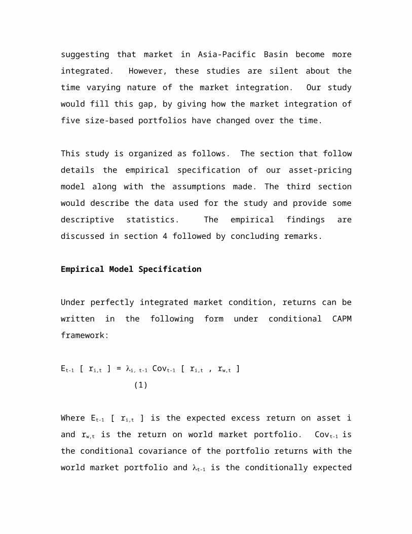
Under perfectly integrated market condition, returns can be written in the following form

under conditional CAPM framework:

Et-1 [ ri,t ] = i, t-1 Covt-1 [ ri,t , rw,t ] (1)

Where Et-1 [ ri,t ] is the expected excess return on asset i and rw,t is the return on world

market portfolio. Covt-1 is the conditional covariance of the portfolio returns with the

world market portfolio and t-1 is the conditionally expected world price of covariance

risk at time t-1 and can be written as the ratio of the excess return on the world market

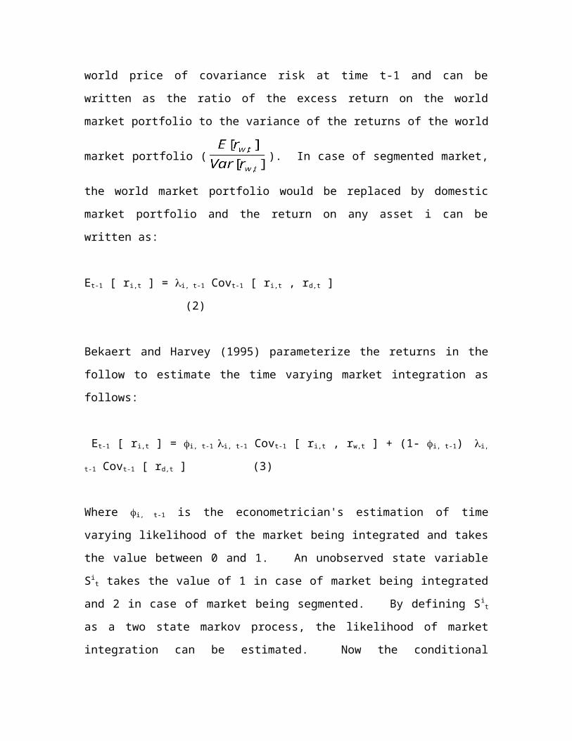
portfolio to the variance of the returns of the world market portfolio ( ). In case

of segmented market, the world market portfolio would be replaced by domestic market

portfolio and the return on any asset i can be written as:

Et-1 [ ri,t ] = i, t-1 Covt-1 [ ri,t , rd,t ] (2)

Bekaert and Harvey (1995) parameterize the returns in the follow to estimate the time

varying market integration as follows:

Et-1 [ ri,t ] = i, t-1 i, t-1 Covt-1 [ ri,t , rw,t ] + (1- i, t-1) i, t-1 Covt-1 [ rd,t ] (3)

Where i, t-1 is the econometrician's estimation of time varying likelihood of the market

being integrated and takes the value between 0 and 1. An unobserved state variable S it

takes the value of 1 in case of market being integrated and 2 in case of market being

segmented. By defining Sit as a two state markov process, the likelihood of market

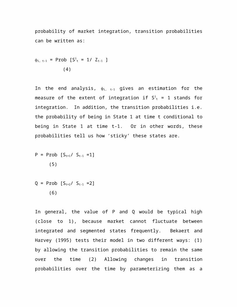
integration can be estimated. Now the conditional probability of market integration,

transition probabilities can be written as:

i, t-1 = Prob [Sit = 1/ Zt-1 ] (4)

In the end analysis, i, t-1 gives an estimation for the measure of the extent of integration if

Sit = 1 stands for integration. In addition, the transition probabilities i.e. the probability of

being in State 1 at time t conditional to being in State 1 at time t-1. Or in other words,

these probabilities tell us how ‘sticky’ these states are.

P = Prob [St=1/ St-1 =1] (5)

Q = Prob [St=2/ St-1 =2] (6)

In general, the value of P and Q would be typical high (close to 1), because market

cannot fluctuate between integrated and segmented states frequently. Bekaert and

Harvey (1995) tests their model in two different ways: (1) by allowing the transition

probabilities to remain the same over the time (2) Allowing changes in transition

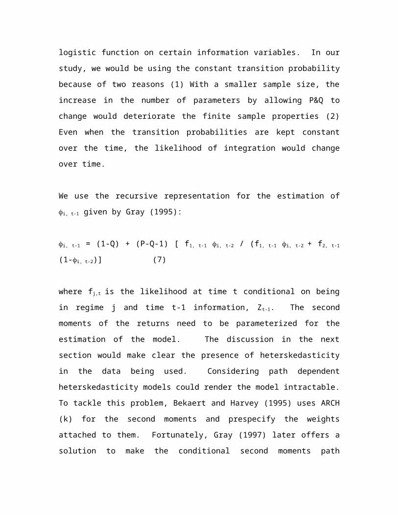
probabilities over the time by parameterizing them as a logistic function on certain

information variables. In our study, we would be using the constant transition probability

because of two reasons (1) With a smaller sample size, the increase in the number of

parameters by allowing P&Q to change would deteriorate the finite sample properties (2)

Even when the transition probabilities are kept constant over the time, the likelihood of

integration would change over time.

We use the recursive representation for the estimation of i, t-1 given by Gray (1995):

i, t-1 = (1-Q) + (P-Q-1) [ f1, t-1 i, t-2 / (f1, t-1 i, t-2 + f2, t-1 (1-i, t-2)] (7)

where fj,t is the likelihood at time t conditional on being in regime j and time t-1

information, Zt-1. The second moments of the returns need to be parameterized for the

estimation of the model. The discussion in the next section would make clear the

presence of heterskedasticity in the data being used. Considering path dependent

heterskedasticity models could render the model intractable. To tackle this problem,

Bekaert and Harvey (1995) uses ARCH (k) for the second moments and prespecify the

weights attached to them. Fortunately, Gray (1997) later offers a solution to make the

conditional second moments path independent and this is used in our GARCH

specification.5 Now our empirical specification can be written as:

Ri, t = [ri,t , rw,t]’ where

(8)

(9)

Define et = [ei,t,ew,t]’ which can be written as:

(10)

The variance and covariance equations are defined in the BEKK format (Baba, Engle,

Kraft and Kroner, 1989) as given below:

(11)

(12)

To reduce the proliferation of number of parameters, we assume that the A,B and C

arrays defined above are symmetric. This reduces the number of parameters to be

estimated to reasonable level. Moreover, the testing is done for individual portfolios thus

optimizing on the number of parameters. This follows from our earlier finding that the

5 For detailed discussion about this problem please refer to page no 34-36 of Gray (1997).

price of risk varies across portfolios. By testing for individual portfolios, we are not

constraining them to be the same for all the portfolios.

The model is estimated using maximum likelihood method and the log likelihood

function can be written as:

where (13)

(14)

(15)

The initial values for the parameters can be defined as the unconditional probability

values or it can be specified as 0.5 (equal probability for integration as well as

segmentation). However, it should be noted that the final distribution is a mixture of two

normal distribution. Hence depending on the mean/variance of the two distributions, it

can have more than one peaks. The typical hill climbing techniques that are used for

maximum likelihood estimation might give us wrong results. Therefore Bekaert and

Harvey (1995) use different sets of initial values to see whether the results obtained are

global optimum.

In additional to doing that, we find out the log likelihood values are behaving for

combinations of initial values. Then these values are plotted as grids and this will show

us the combination of initial values for which the log likelihood values are global

optimum. In our case, we found that the log likelihood values are more sensitive to the

initial values of the transitional probabilities and hence different combination of

transition probabilities are used to find the global optimum.

Specification Tests and Diagnostics

To test the performance of the model, we regress the disturbance vector et on the

information available at time T-1. In our case, we can consider the returns at time T-1 as

the information variable. For the model to be performing well, the disturbance vector

should be orthogonal to the lagged returns. The diagnostic tests consider the R2 obtained

from the regression and the Wald statistic for the joint testing of all the coefficients

obtained from the regression.

Data Description and Summary Statistics

We use monthly data from 1990:01 - 2001:12 for 100 stocks listed in Bombay Stock

Exchange during the period 1990-2001. These 100 stocks are selected based on the

following criteria: (1) The stocks selected should have been listed in Bombay Stock

Exchange for the entire period 1990:01 - 2001:12. (2) There should be at least one

trading in every month during the time period. (3) The final 100 stocks were selected

based on the number of trading days. Five value-weighted portfolios were constructed by

value ranking of the companies on the basis of market capitalization at the end of every

year and splitting these companies into value-ranked quintiles, and then forming five

portfolios based on value weights within a quintile.

The monthly adjusted closing price data for the stocks were collected from the data

published by the 'Centre for Monitoring Indian Economy' (CMIE). The call money rate

published by the Reserve Bank of India (2001) was used as the short term risk free rate6.

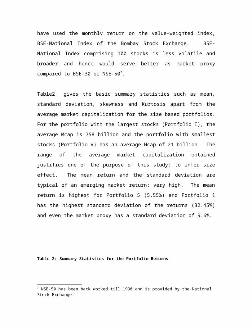
For the market return, we have used the monthly return on the value-weighted index,

BSE-National Index of the Bombay Stock Exchange. BSE-National Index comprising

100 stocks is less volatile and broader and hence would serve better as market proxy

compared to BSE-30 or NSE-507.

Table2 gives the basic summary statistics such as mean, standard deviation, skewness

and Kurtosis apart from the average market capitalization for the size based portfolios.

6 Three-month treasury bill rates are generally used for this purpose. Since it is not available for the whole period call money rates have been used.7 NSE-50 has been back worked till 1990 and is provided by the National Stock Exchange.

For the portfolio with the largest stocks (Portfolio I), the average Mcap is 758 billion and

the portfolio with smallest stocks (Portfolio V) has an average Mcap of 21 billion. The

range of the average market capitalization obtained justifies one of the purpose of this

study: to infer size effect. The mean return and the standard deviation are typical of an

emerging market return: very high. The mean return is highest for Portfolio 5 (5.55%)

and Portfolio 1 has the highest standard deviation of the returns (32.45%) and even the

market proxy has a standard deviation of 9.6%.

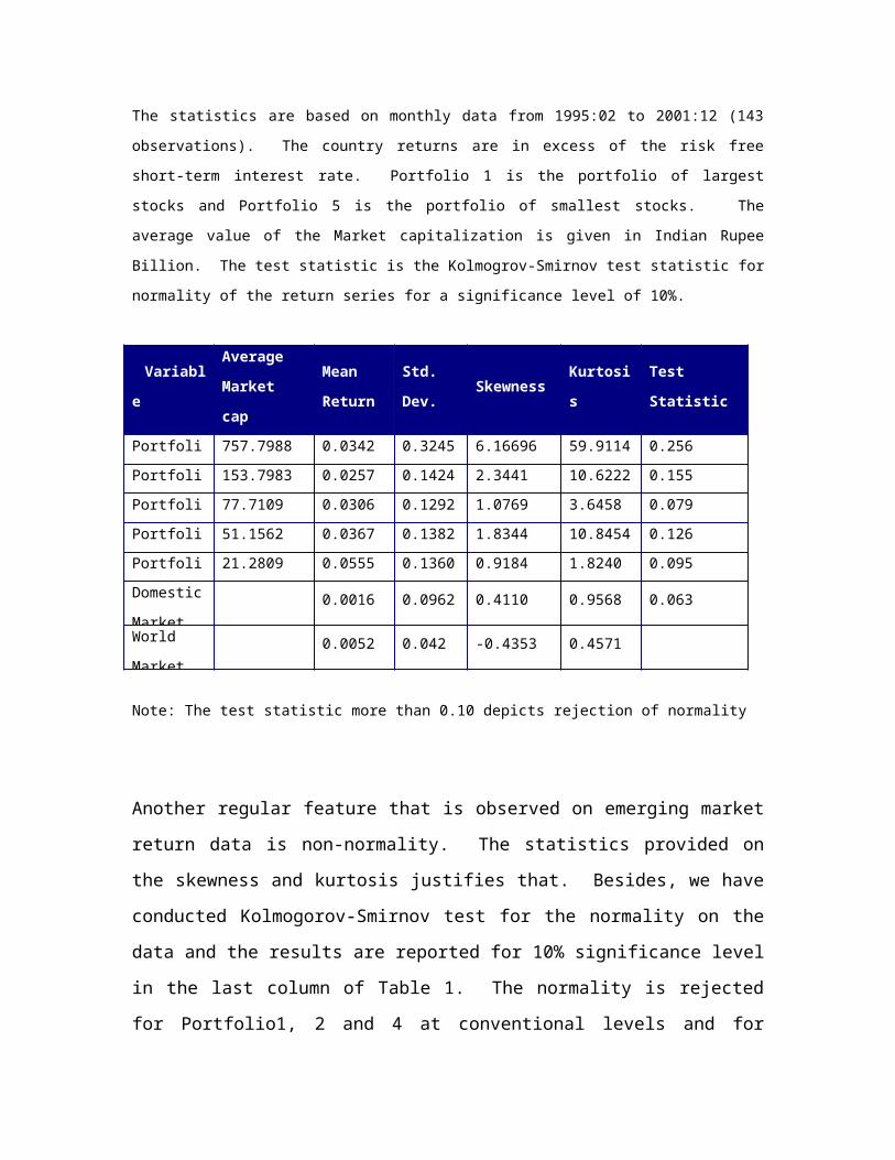
Table 2: Summary Statistics for the Portfolio Returns

The statistics are based on monthly data from 1995:02 to 2001:12 (143 observations). The country returns are in excess of the risk free short-term interest rate. Portfolio 1 is the portfolio of largest stocks and Portfolio 5 is the portfolio of smallest stocks. The average value of the Market capitalization is given in Indian Rupee Billion. The test statistic is the Kolmogrov-Smirnov test statistic for normality of the return series for a significance level of 10%.

VariableAverage Market cap

Mean Return

Std. Dev.

Skewness

Kurtosis

Test Statistic

Portfolio 1

757.7988 0.0342 0.3245 6.16696 59.9114 0.256Portfolio 2

153.7983 0.0257 0.1424 2.3441 10.6222 0.155Portfolio 3

77.7109 0.0306 0.1292 1.0769 3.6458 0.079Portfolio 4

51.1562 0.0367 0.1382 1.8344 10.8454 0.126Portfolio 5

21.2809 0.0555 0.1360 0.9184 1.8240 0.095Domestic Market

0.0016 0.0962 0.4110 0.9568 0.063

World Market

0.0052 0.042 -0.4353 0.4571

Note: The test statistic more than 0.10 depicts rejection of normality

Another regular feature that is observed on emerging market return data is non-normality.

The statistics provided on the skewness and kurtosis justifies that. Besides, we have

conducted Kolmogorov-Smirnov test for the normality on the data and the results are

reported for 10% significance level in the last column of Table 1. The normality is

rejected for Portfolio1, 2 and 4 at conventional levels and for Portfolio 3, 5 and the

market return they are rejected at 5% significance level. This justifies our use of

Generalized Method of Moments (GMM) procedure to estimate the model.

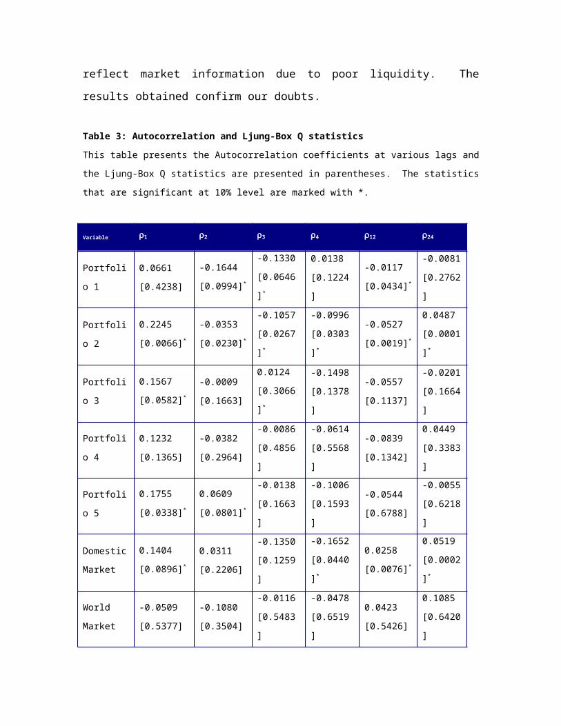
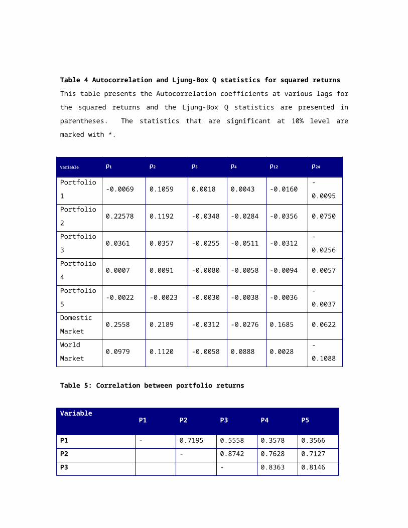
Table 3 and Table 4 reports the auto correlation properties of the returns, as well as the

correlation between the portfolio returns and the instrumental variables respectively. The

autocorrelation coefficients and the Ljung-Box Q statistics provide evidence that the

Indian stock returns are highly persistent. The correlation between portfolio returns and

the market in Table 4 reveals high correlation but counter intuitive. Portfolio 1 has the

lower correlation coefficient (0.50) with the market compared to smaller stock portfolios.

One would expect larger stock to move more closely with the market. This could be

because our Portfolio 1 is more volatile compared to the market proxy, which is a value-

weighted index of 100 stocks.

The cross correlation between the portfolios are also very high (Table 3). It also reveals

another interesting detail. The strength of correlation with other portfolios decreases with

the decrease in size. To understand this more we find the cross correlation coefficients

with lags because it is quite possible that the larger stocks reflect market information

quickly and smaller stocks take more time to reflect market information due to poor

liquidity. The results obtained confirm our doubts.

Table 3: Autocorrelation and Ljung-Box Q statisticsThis table presents the Autocorrelation coefficients at various lags and the Ljung-Box Q statistics are presented in parentheses. The statistics that are significant at 10% level are marked with *.

Variable 1 2 3 4 12 24

Portfolio 1

0.0661[0.4238]

-0.1644[0.0994]*

-0.1330[0.0646]*

0.0138[0.1224]

-0.0117[0.0434]*

-0.0081[0.2762]

Portfolio 2

0.2245[0.0066]*

-0.0353[0.0230]*

-0.1057[0.0267]*

-0.0996[0.0303]*

-0.0527[0.0019]*

0.0487[0.0001]*

Portfolio 3

0.1567[0.0582]*

-0.0009[0.1663]

0.0124[0.3066]*

-0.1498[0.1378]

-0.0557[0.1137]

-0.0201[0.1664]

Portfolio 4

0.1232[0.1365]

-0.0382[0.2964]

-0.0086[0.4856]

-0.0614[0.5568]

-0.0839[0.1342]

0.0449[0.3383]

Portfolio 5

0.1755[0.0338]*

0.0609[0.0801]*

-0.0138[0.1663]

-0.1006[0.1593]

-0.0544[0.6788]

-0.0055[0.6218]

Domestic Market

0.1404[0.0896]*

0.0311[0.2206]

-0.1350[0.1259]

-0.1652[0.0440]*

0.0258[0.0076]*

0.0519[0.0002]*

World Market

-0.0509[0.5377]

-0.1080[0.3504]

-0.0116[0.5483]

-0.0478[0.6519]

0.0423[0.5426]

0.1085[0.6420]

Table 4 Autocorrelation and Ljung-Box Q statistics for squared returnsThis table presents the Autocorrelation coefficients at various lags for the squared returns and the Ljung-Box Q statistics are presented in parentheses. The statistics that are significant at 10% level are marked with *.

Variable 1 2 3 4 12 24

Portfolio 1 -0.0069 0.1059 0.0018 0.0043 -0.0160 -0.0095Portfolio 2 0.22578 0.1192 -0.0348 -0.0284 -0.0356 0.0750Portfolio 3 0.0361 0.0357 -0.0255 -0.0511 -0.0312 -0.0256Portfolio 4 0.0007 0.0091 -0.0080 -0.0058 -0.0094 0.0057Portfolio 5 -0.0022 -0.0023 -0.0030 -0.0038 -0.0036 -0.0037Domestic Market

0.2558 0.2189 -0.0312 -0.0276 0.1685 0.0622

World 0.0979 0.1120 -0.0058 0.0888 0.0028 -0.1088

Market

Table 5: Correlation between portfolio returns

VariableP1 P2 P3 P4 P5

P1 - 0.7195 0.5558 0.3578 0.3566P2 - 0.8742 0.7628 0.7127P3 - 0.8363 0.8146P4 - 0.8488P5 -Market Proxy 0.5040 0.7847 0.8265 0.8092 0.7679

Empirical Results

This section discusses the empirical estimation of the likelihood of integration of the size

based portfolio. As mentioned above, the parameters are estimated using the grid

approach. Appendix 1 gives the changes in the P, Q and for various combinations of

initial parameters. We have varied P & Q systematically over the range 0.9 to 0.99 with

small increments (0.3) to estimate value of the likelihood function. The range of 0.9 to

0.99 is used because the transition probabilities are expected to be in the higher range

because the markets cannot switch between integrated and segmented states quite

frequently. The initial value for is given as 0.5, which means that there, is equal chance

for being in integrated state as well as segmented state (Please also see foot note 8). The

maximum value of likelihood function obtained through the step described above is given

in the tables given below8.

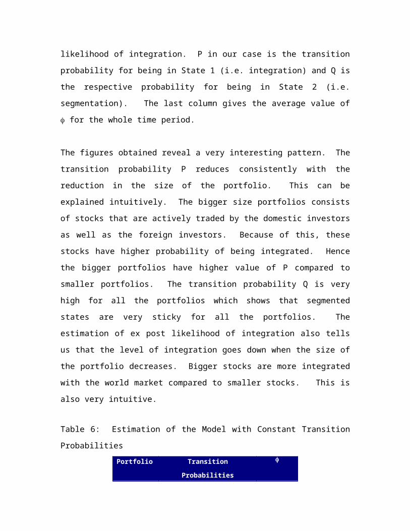
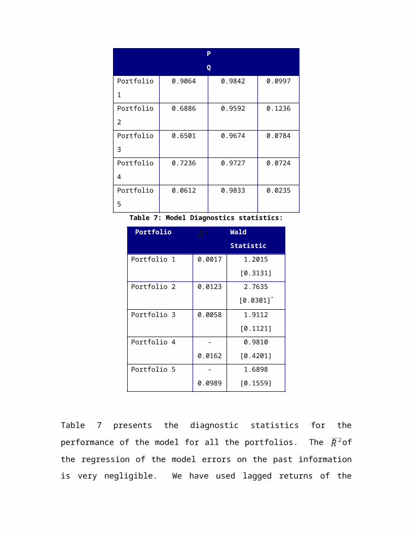
Table 6 presents the estimation of the transition probability (P & Q) along with the

estimation of the likelihood of integration. P in our case is the transition probability for

being in State 1 (i.e. integration) and Q is the respective probability for being in State 2

8 As a further refinement, for this combination of P & Q, we then change the initial estimate of and see whether there is change in the likelihood function. Change of do not have much impact on increasing the value of the likelihood function.

(i.e. segmentation). The last column gives the average value of for the whole time

period.

The figures obtained reveal a very interesting pattern. The transition probability P

reduces consistently with the reduction in the size of the portfolio. This can be explained

intuitively. The bigger size portfolios consists of stocks that are actively traded by the

domestic investors as well as the foreign investors. Because of this, these stocks have

higher probability of being integrated. Hence the bigger portfolios have higher value of P

compared to smaller portfolios. The transition probability Q is very high for all the

portfolios which shows that segmented states are very sticky for all the portfolios. The

estimation of ex post likelihood of integration also tells us that the level of integration

goes down when the size of the portfolio decreases. Bigger stocks are more integrated

with the world market compared to smaller stocks. This is also very intuitive.

Table 6: Estimation of the Model with Constant Transition Probabilities

Portfolio Transition ProbabilitiesP Q

Portfolio 1 0.9064 0.9842 0.0997Portfolio 2 0.6886 0.9592 0.1236Portfolio 3 0.6501 0.9674 0.0784Portfolio 4 0.7236 0.9727 0.0724Portfolio 5 0.0612 0.9833 0.0235

Table 7: Model Diagnostics statistics: Portfolio Wald

StatisticPortfolio 1 0.0017 1.2015

[0.3131]Portfolio 2 0.0123 2.7635

[0.0301]*

Portfolio 3 0.0058 1.9112[0.1121]

Portfolio 4 -0.0162 0.9810[0.4201]

Portfolio 5 -0.0989 1.6898

[0.1559]

Table 7 presents the diagnostic statistics for the performance of the model for all the

portfolios. The of the regression of the model errors on the past information is very

negligible. We have used lagged returns of the portfolios as the past information because

as per the assumptions of our model, the model errors should be orthogonal to the past

returns. The last column provides wald statistic for the joint hypothesis that coefficients

obtained from the above regression is zero. The wald statistics also confirm that the

regression coefficients obtained are not significantly different from zero.

Figure 1: Plot of likelihood of market integration

Portfolio 1

1990 1991 1992 1993 1994 1995 1996 1997 1998 1999 2000 20010.00

0.25

0.50

0.75

1.00

Portfolio 2

1990 1991 1992 1993 1994 1995 1996 1997 1998 1999 2000 20010.0

0.1

0.2

0.3

0.4

0.5

0.6

0.7

Portfolio 3

1990 1991 1992 1993 1994 1995 1996 1997 1998 1999 2000 20010.0

0.1

0.2

0.3

0.4

0.5

0.6

0.7

Portfolio 4

1990 1991 1992 1993 1994 1995 1996 1997 1998 1999 2000 20010.00

0.25

0.50

0.75

Portfolio 5

1990 1991 1992 1993 1994 1995 1996 1997 1998 1999 2000 20010.016648

0.016656

0.016664

0.016672

0.016680

0.016688

0.016696

Figure 1 gives a plot on how the level of integration changes over time. The plots for

Portfolio 1 and Portfolio 2 looks similar to the plot obtained by Bekaert and Harvey

(1995) for the period up to 1995. For Portfolio 1,2 and 3 (larger stock portfolios) show

that they are integrated with the world market during the year 1994. It may be noted that

that active participation of foreign portfolio investments in India started during this

period only. Also Portfolio 1 and Portfolio 2 shows a spike during the 1992. This period

coincides with the securities market scam in India and the stocks comprising Portfolio 1

and 2 showed witnessed extreme volatility.

Another important event that did not have any significant impact conspicuously on the

level of integration is the South East Asian Crisis during 1997. Though the quantum of

foreign portfolio investments to Indian capital market have increased multifold post

South Asian crisis that does not seem to have impact on the level of integration.

Conclusion

We have attempted to estimate the likelihood of integration of size-based portfolios of

Indian stocks with the world market using markov regime switching model. Given

smaller sample size and lesser likelihood of integration, we use a grid approach to

estimate the maximum likelihood estimates. We find that that there is a clear pattern on

the integration of size based portfolios. The transition probability of being in integrated

state and the average level of integration decrease with the reduction in the size of the

portfolios. Also the segmented state seems to be a very sticky stage. Plot of time varying

integration of these portfolios were drawn and it was checked whether the periods of

higher integration coincide with any of major mile stone event in the Indian /International

capital market.

ReferencesAlexander, G J., Eun, C. S. and Janakiraman, S., 1988, "International listings and stock

returns: some empirical evidence", Journal of financial and Quantitative analysis, 23,

135-51.

Baba, Yoshihisa, Robert F. Engle, Dennis F. Kraft and Kenneth F. Kroner, 1989,

“Multivariate simultaneous generalized ARCH”, working paper, University of California,

San Diego, California.

Bekaert, Geert, and Robert Hodrick, 1992, “Characterizing predictable components in

excess returns on equity and foreign exchange markets”, Journal of Finance, 47, 467-509

Bekaert, G. and Harvey, Campbell R, 1995, "Time-Varying World Market Integration",

Journal of Finance, 50, 2, 403-445.

Bekaert, G, and Harvey, Campbell R, 2000, "Foreign speculators and emerging equity

markets", Journal of Finance, 55, 2, 565-614.

Bekaert, Geert, Harvey, Campbell, R., and Robin Lumsdaine, 2002, “ Dating the

integration of world capital markets”, Journal of Financial Economics, 65:2, 2002, 203-

249

Black, F., 1972, "Capital Market Equilibrium with Restricted Borrowing", Journal of

Business, 45, July, 444-454.

Campbell, John Y., and Yasushi Hamao,1989, “Predictable bond and stock returns in the

United States and Japan: A study of long-term capital market integration”, working

paper, Princeton University.

Campbell, J.Y., and J.H.Hentschel, 1992, "No News is Good News: An Asymmetric

Model of Changing Volatility in Stock Returns", Journal of Financial Economics, 31,

281-318.

Cho, Chinhyung D., Cheol S. Eun and Lemma W. Senbet, 1986, “International arbitrage

pricing theory: An empirical investigation”, Journal of Finance, 41, 313-330

Choe, Hyuk, Kho, Bong-Chan and Stulz, R.M., 1998, "Do foreign investors destabilize

stock markets - The Korean experience in 1997", NBER working paper.

Domowitz, I, Glen J and Madhavan, A., 1997, "Market Segmentation and Stock Prices:

Evidence from an Emerging Market", Journal of Finance, 52, 1059-1085.

Dumas, Bernard and Bruno, Solnik, 1995, “The world price of foreign price risk”,

Journal of Finance, 50, 445-479.

Errunza, V. and Losq, E., 1985, "International asset pricing under mile segmentation:

theory and test", Journal of Finance, 40, 105-24.

Errunza, V. and Losq, E., 1989, "Capital flow controls, international asset pricing, and

investors’ welfare: a multi country framework", Journal of Finance, 44, 1025-38.

Eun, C.S. and Janakiraman, S., 1986, "A model of international asset pricing with a

constraint on the foreign equity ownership", Journal of Finance, 41, 897-914.

Ferson, Wayne E., and Harvey, Campbell, Harvey, R., 1993, “The risk and predictability

of international equity returns, Review of Financial Studies, 6, 527-566.

Ferson, Wayne E., and Harvey, Campbell, Harvey, R., 1994a, “Sources of risk and

expected returns in global equity markets”, Journal of Banking and Finance, 18, 775-

803.

Ferson, Wayne E., and Harvey, Campbell, Harvey, R., 1994b, “An exploratory

investigation of the fundamental determinants of national equity market returns, in

Jeffrey Frankel Ed.: The Internationalization of Equity Markets, University of Chicago

Press, Chicago, IL, 59-138

Gray, Stephen F., 1995, “An analysis of conditional regime switching models”, working

paper, Duke University.

Gray, Stephen F., 1997, “Modeling the conditional distribution of interest rates as a

regime-switching process”, Journal of Financial Economics, 42, 27-62.

Harvey, Campbell R., 1991, “The world price of covariance risk”, The Journal of

Finance 46, 111-157.

Henry, Peter B., 2000a, Stock Market Liberalization, Economic Reform and Emerging

Equity Prices, Journal of Finance, 55,2, 529-564.

Henry, Peter B., 2000b, "Do Stock Market Liberalizations Cause Investment Booms?",

Journal of Financial Economics, 58, 301-334.

Kim, E. Han and Singhal, Vijay, 2000, Stock Market Openings: Experience of Emerging

Economies, Journal of Business, 73, 1, 25-66.

.Harvey, Campbell R., Bruno, H., Solnik and Guofu Zhou, 1994, “What determines

expected international asset returns?”, Working paper, Duke University, Durham, N.C.

Kiran, K.K. and Mukhopadyay C., 2002, " Equity Market Interlinkages: Transmission of

volatility a case study of US and India", NSE research initiative, Paper No. 16.

Pradhan, H.K., and Narasimhan, S.L, 2003, Stock Price Behavior in India since

liberalization, Asia-Pacific Development Journal, 9, 83-106.

Shah, Ajay and Sivkumar, Sivaprakasam, 2000, “Changing Liquidity in the Indian equity

market”, Emerging Markets Quarterly, 4(2), Summer 2000, 62-71.

Solnik, Bruno, 1983, “The relationship between stock prices and inflationary

expectations: The international evidence”, Journal of Finance, 38, 35-48.

Stulz, Rene, 1981, “A model of international asset pricing”, Journal of Financial

Economics, 9, 383-406.

Wheatley, Simon, 1988, “Some tests of international equity integration”, Journal of

Financial Economics, 21, 177-212.

Annexure 1 – Grid Approach for finding Maximum Likelihood Estimators

Description of Portfolio

Initial Values Estimated Values

Portfolio 1

P Q P Q LikelihoodFunction

0.900.90 0.813 0.974 799.6190.93 0.808 0.974 765.3050.96 0.840 0.974 795.8820.99 0.796 0.974 798.316

0.93

0.90 0.9064 0.984 800.1200.93 0.8252 0.974 796.0270.96 0.8343 0.974 797.9380.99 0.8150 0.975 796.856

0.96

0.90 0.832 0.975 796.8170.93 0.820 0.974 797.6500.96 0.799 0.975 799.3360.99 0.805 0.974 797.491

0.99

0.90 0.823 0.974 797.6610.93 0.824 0.974 796.9110.96 0.797 0.974 797.1230.99 0.816 0.975 795.371

Description of Portfolio

Initial Values Estimated Values

Portfolio 2

P Q P Q LikelihoodFunction

0.900.90 0.720 0.963 738.0590.93 0.704 0.964 740.1790.96 0.703 0.961 741.5400.99 0.708 0.960 738.833

0.93

0.90 0.726 0.963 737.2840.93 0.718 0.960 742.1930.96 0.688 0.959 742.2520.99 0.493 0.933 736.385

0.96

0.90 0.713 0.956 741.5100.93 0.715 0.957 741.8680.96 0.718 0.962 737.8060.99 0.681 0.960 740.268

0.99

0.90 0.717 0.801 739.9730.93 0.717 0.860 740.8760.96 0.699 0.950 739.5210.99 0.728 0.956 739.398

Description of Portfolio

Initial Values Estimated Values

P Q P Q LikelihoodFunction

0.900.90 0.525 0.979 698.6880.93 0.334 0.971 698.1140.96 0.547 0.972 698.3790.99 0.623 0.965 702.890

0.93

0.90 0.602 0.965 699.4940.93 0.389 0.866 698.8970.96 0.243 0.930 690.4500.99 0.565 0.978 699.441

Portfolio 3

0.96

0.90 0.549 0.967 698.8850.93 0.535 0.960 700.6810.96 0.547 0.959 700.3090.99 0.650 0.967 703.559

0.99

0.90 0.535 0.968 699.1760.93 0.574 0.974 699.6690.96 0.403 0.973 701.1500.99 0.376 0.972 699.741

Description of Portfolio Initial Values Estimated Values

Portfolio 4

P Q P Q LikelihoodFunction

0.800.80 0.680 0.979 691.4880.83 0.178 0.898 688.6070.86 0.517 0.978 688.6770.89 0.695 0.982 687.081

0.83

0.80 0.608 0.978 687.7150.830.86 0.622 0.973 684.1980.89 0.401 0.967 685.740

0.8

0.80 0.63 0.988 690.4960.83 0.168 0.989 691.4950.86 0.723 0.972 698.8300.89 0.624 0.979 690.444

Portfolio 5

0.80 0.80 0.367 0.996 665.7550.80 0.86 0.050 0.984 682.4940.70 0.70 0.0313 0.988 681.0050.70 0.95 0.0612 0.9833 683.982