arthurcharpentier - f-origin.hypotheses.org · arthur charpentier, master université rennes 1 -...
TRANSCRIPT
Arthur Charpentier, Master Université Rennes 1 - 2017
Arthur Charpentier
https://freakonometrics.github.io/
Université Rennes 1, 2017
Probability & Statistics
@freakonometrics freakonometrics freakonometrics.hypotheses.org 1
Arthur Charpentier, Master Université Rennes 1 - 2017
Agenda
Introduction: Statistical Model• Probability Usual notations, P, F , f , E, Var Usual distributions: discrete & continuous Conditional Distribution, Conditional Expectation, Mixtures Convergence, Approximation and Asymptotic Results
· Law of Large Numbers (LLN)· Central Limit Theorem (CLT)
• (Mathematical Statistics) From descriptive statistics to mathematical statistics Sampling: mean and variance Confidence Interval Decision Theory and Testing Procedures
@freakonometrics freakonometrics freakonometrics.hypotheses.org 2
Arthur Charpentier, Master Université Rennes 1 - 2017
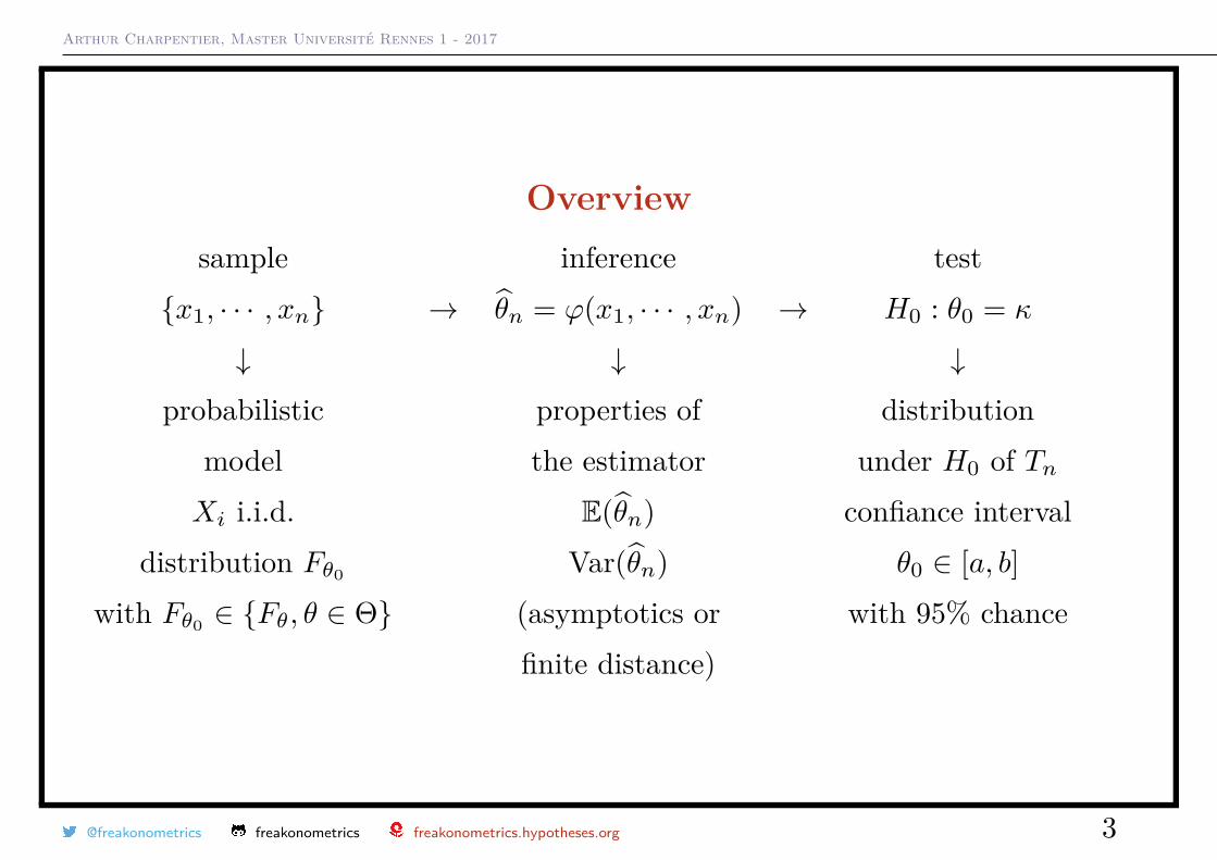
Overviewsample inference test
x1, · · · , xn → θn = ϕ(x1, · · · , xn) → H0 : θ0 = κ
↓ ↓ ↓probabilistic properties of distribution
model the estimator under H0 of TnXi i.i.d. E(θn) confiance interval
distribution Fθ0 Var(θn) θ0 ∈ [a, b]with Fθ0 ∈ Fθ, θ ∈ Θ (asymptotics or with 95% chance
finite distance)
@freakonometrics freakonometrics freakonometrics.hypotheses.org 3
Arthur Charpentier, Master Université Rennes 1 - 2017
Additional ReferencesAbebe, Daniels & McKean (2001) Statistics and Data Analysis
Freedman (2009) Statistical Models: Theory and Practice. Cambridge UniversityPress.
Grinstead & Snell (2015) Introduction to Probability
Hogg, McKean & Craig (2005) Introduction to Mathematical Statistics.Cambridge University Press.
Kerns (2010) Introduction to Probability and Statistics Using R.
@freakonometrics freakonometrics freakonometrics.hypotheses.org 4
Arthur Charpentier, Master Université Rennes 1 - 2017
Probability SpaceAssume that there is a probability space (Ω,A,P).
• Ω is the fundamental space: Ω = ωi, i ∈ I is the set of all results from arandom experiment.
• A is the σ-algebra of evevents, ie the set of all parts of Ω.• P is a probability measure on Ω, i.e.
P(Ω) = 1 for any event A in Ω, 0 ≤ P(A) ≤ 1, for any A1, · · · , An mutually exclusive (Ai ∩Aj = ∅),
P(n⋃i=1
Ai) =n∑i=1
P(Ai)
A random variable X is a function Ω→ R.
@freakonometrics freakonometrics freakonometrics.hypotheses.org 5
Arthur Charpentier, Master Université Rennes 1 - 2017
Probability SpaceOne flip of a fair coin: the outcome is either heads or tails, Ω = H,T, e.g.ω = H ∈ Ω.
The σ-algebra is A = , H, T, H,T, or F = ∅, H, T,Ω
There is a fifty percent chance of tossing heads and fifty percent for tails,P() = 0, P(H) = 0.5 P(T) = 0.5 and P(H,T) = 1.
Consider a game where we gain 1 if the outcome is head, 0 otherwise. Let Xdenote our financial income. X is a random variable with values 0, 1.P(X = 0) = 0.5 and P(X = 1) = 0.5 is the distribution of X on 0, 1.
@freakonometrics freakonometrics freakonometrics.hypotheses.org 6
Arthur Charpentier, Master Université Rennes 1 - 2017
Probability Spacen flip of a fair coin, the outcome is either heads or tails, each time, Ω = H,Tn,e.g. ω = H,H, T, · · · , T,H ∈ Ω.
The σ-algebra is A = , H, T, H,H, H,T, T,H, · · · .
There is a fifty percent chance of tossing heads and fifty percent for tails,P (ω) = 0 if #ω 6= n, otherwise, probability is 1/2n,
P(H,H, T, · · · , T,H) = 12n
Consider a game where we gain 1 if the outcome is head, 0 otherwise. Let Xdenote our financial income. X is a random variable with values 0, 1, · · · , n (Xis also the number of heads obtained out of n draws). P (X = 0) = 1/2n,P (X = 1) = n/2n, etc, is the distribution of X on 0, 1, · · · , n.
@freakonometrics freakonometrics freakonometrics.hypotheses.org 7
Arthur Charpentier, Master Université Rennes 1 - 2017
Usual FunctionsDefinition Let X denote a random variable, its cumulative distribution function(cdf) is
F (x) = P(X ≤ x), for all x ∈ R.
More formally, F (x) = P(ω ∈ Ω|X(ω) ≤ x).
Observe that
• F is an increasing function on R with values in [0, 1],• limx→−∞
F (x) = 0 and limx→+∞
F (x) = 1.
X and Y are equal in distribution, denoted X L= Y if for any x
FX(x) = P(X ≤ x) = P(Y ≤ x) = FY (x).
The survival function is F (x) = 1− F (x) = P(X > x).
@freakonometrics freakonometrics freakonometrics.hypotheses.org 8
Arthur Charpentier, Master Université Rennes 1 - 2017
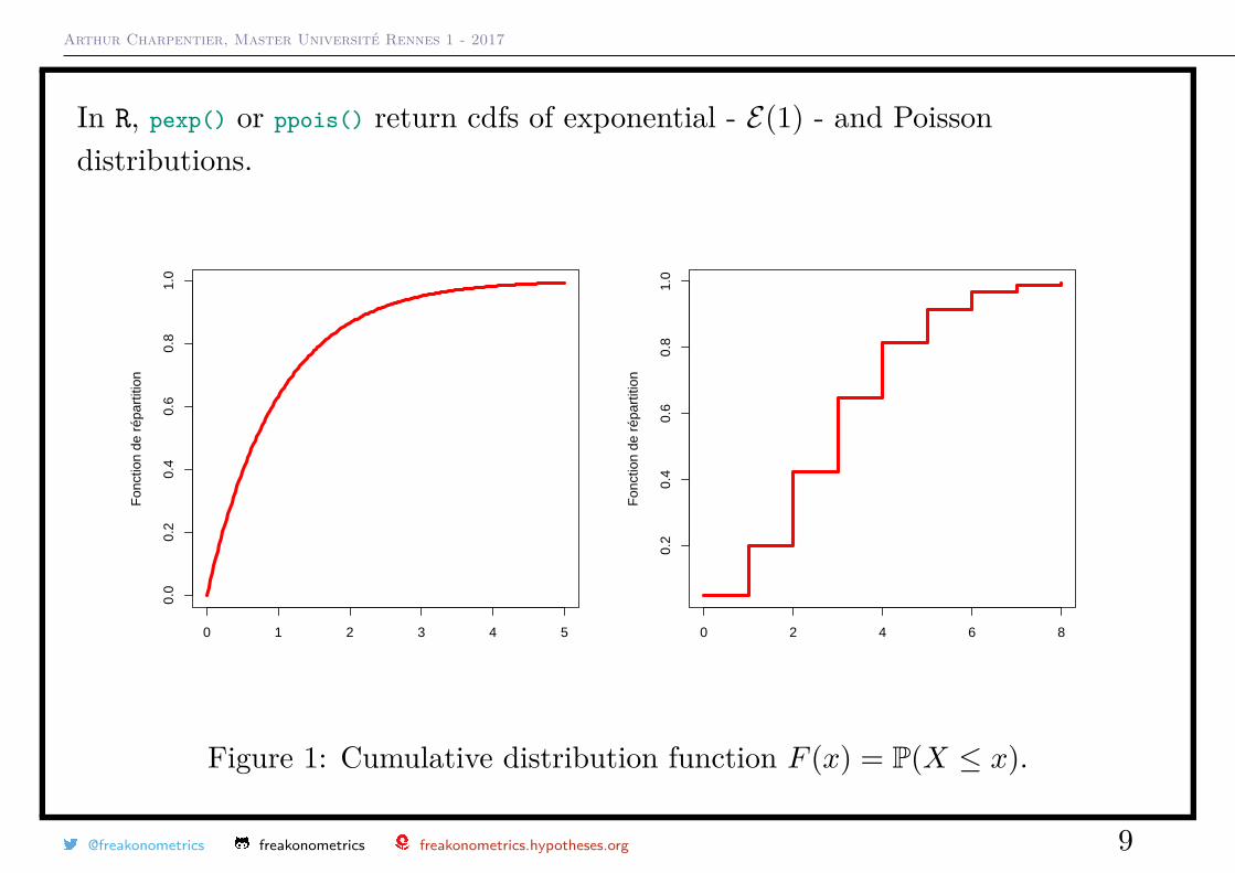
In R, pexp() or ppois() return cdfs of exponential - E(1) - and Poissondistributions.
0 1 2 3 4 5
0.0
0.2
0.4
0.6
0.8
1.0
Fon
ctio
n de
rép
artit
ion
0 2 4 6 8
0.2
0.4
0.6
0.8
1.0
Fon
ctio
n de
rép
artit
ion
Figure 1: Cumulative distribution function F (x) = P(X ≤ x).
@freakonometrics freakonometrics freakonometrics.hypotheses.org 9
Arthur Charpentier, Master Université Rennes 1 - 2017
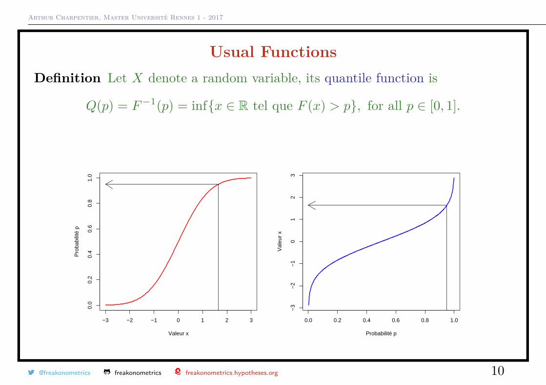
Usual FunctionsDefinition Let X denote a random variable, its quantile function is
Q(p) = F−1(p) = infx ∈ R tel que F (x) > p, for all p ∈ [0, 1].
−3 −2 −1 0 1 2 3
0.0
0.2
0.4
0.6
0.8
1.0
Valeur x
Pro
babi
lité
p
0.0 0.2 0.4 0.6 0.8 1.0
−3
−2
−1
01
23
Probabilité p
Val
eur
x
@freakonometrics freakonometrics freakonometrics.hypotheses.org 10

Arthur Charpentier, Master Université Rennes 1 - 2017
With R, qexp() and qpois() are quantile functions of the exponential (E(1)) andthe Poisson distribution.
0.0 0.2 0.4 0.6 0.8 1.0
01
23
45
6
Fon
ctio
n qu
antil
e
0.0 0.2 0.4 0.6 0.8 1.0
02
46
8
Fon
ctio
n qu
antil
e
Figure 2: Quantile function Q(p) = F−1(p).
@freakonometrics freakonometrics freakonometrics.hypotheses.org 11
Arthur Charpentier, Master Université Rennes 1 - 2017
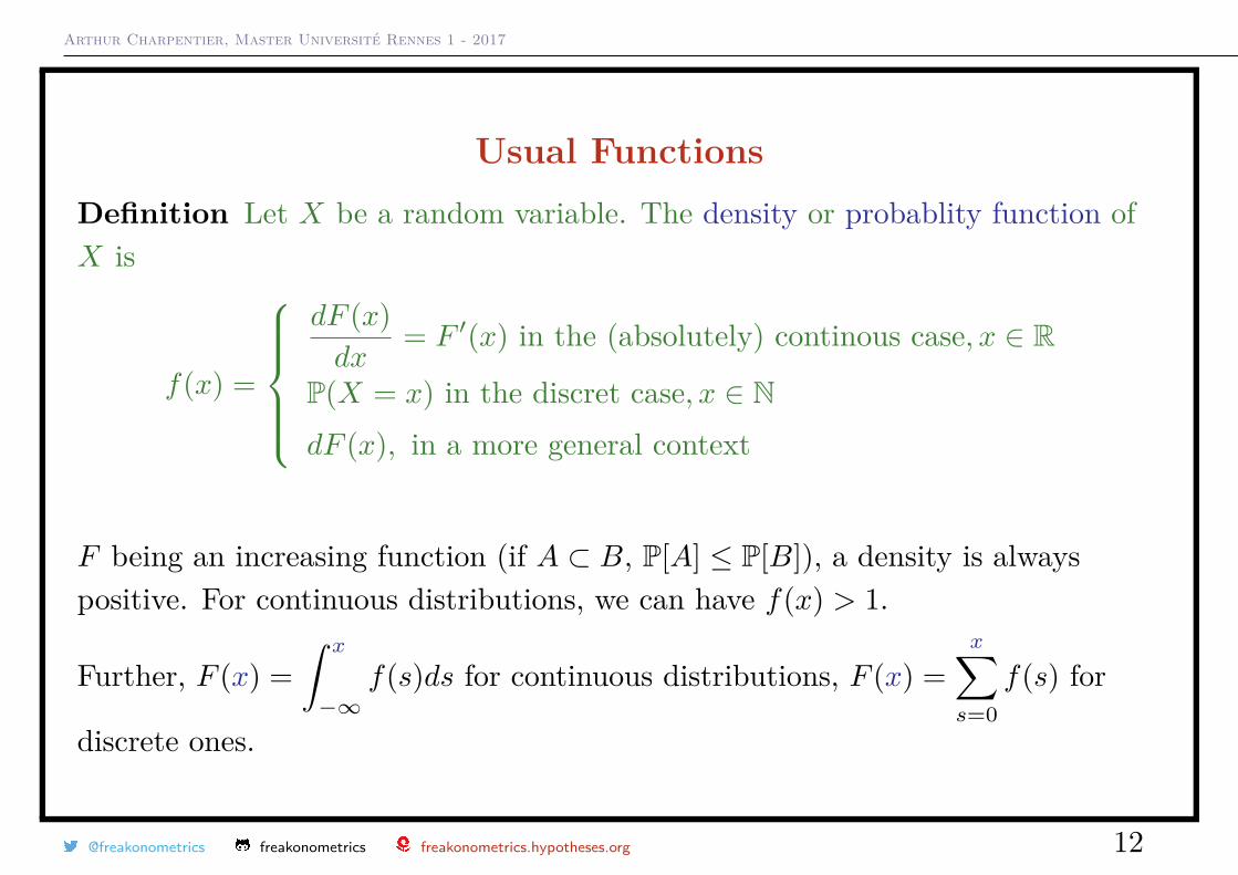
Usual FunctionsDefinition Let X be a random variable. The density or probablity function ofX is
f(x) =
dF (x)dx
= F ′(x) in the (absolutely) continous case, x ∈ R
P(X = x) in the discret case, x ∈ N
dF (x), in a more general context
F being an increasing function (if A ⊂ B, P[A] ≤ P[B]), a density is alwayspositive. For continuous distributions, we can have f(x) > 1.
Further, F (x) =∫ x
−∞f(s)ds for continuous distributions, F (x) =
x∑s=0
f(s) for
discrete ones.
@freakonometrics freakonometrics freakonometrics.hypotheses.org 12
Arthur Charpentier, Master Université Rennes 1 - 2017
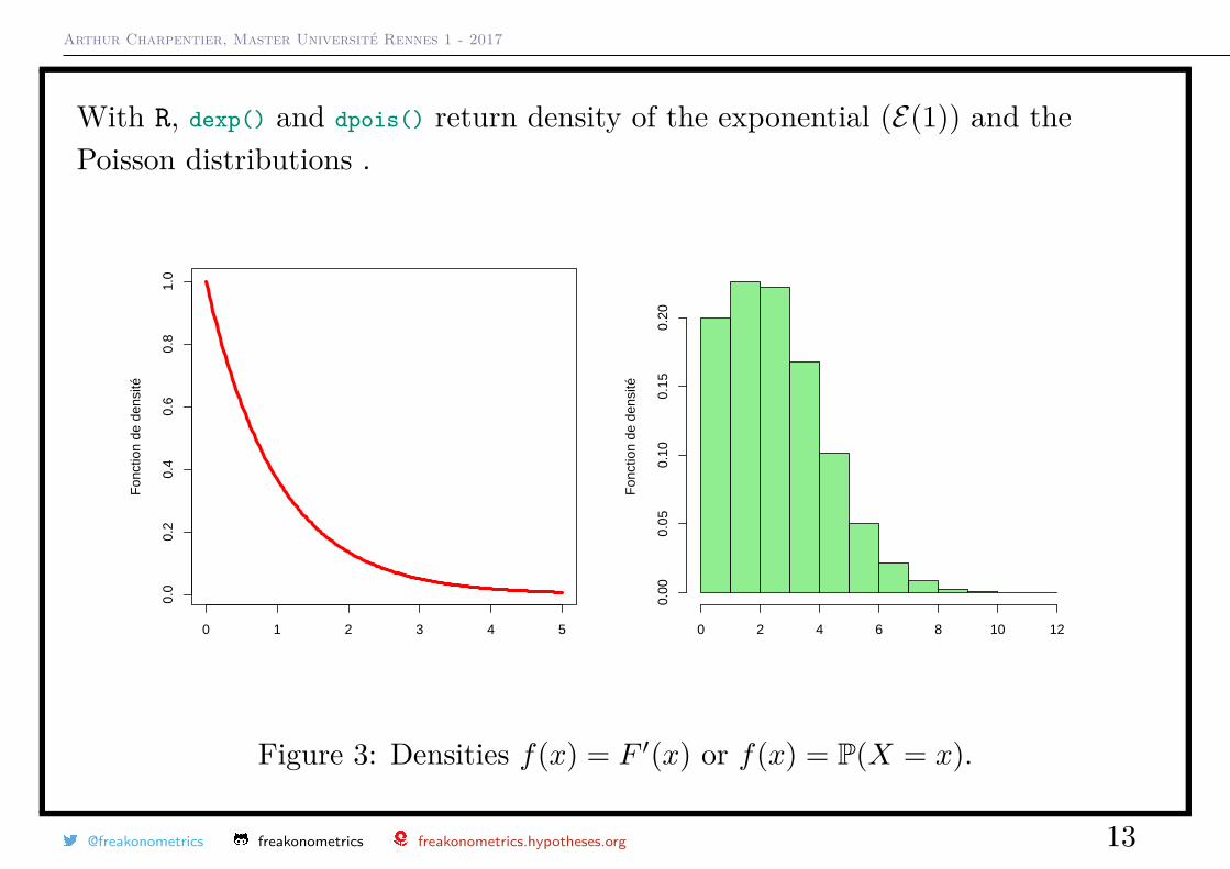
With R, dexp() and dpois() return density of the exponential (E(1)) and thePoisson distributions .
0 1 2 3 4 5
0.0
0.2
0.4
0.6
0.8
1.0
Fon
ctio
n de
den
sité
Fon
ctio
n de
den
sité
0 2 4 6 8 10 12
0.00
0.05
0.10
0.15
0.20
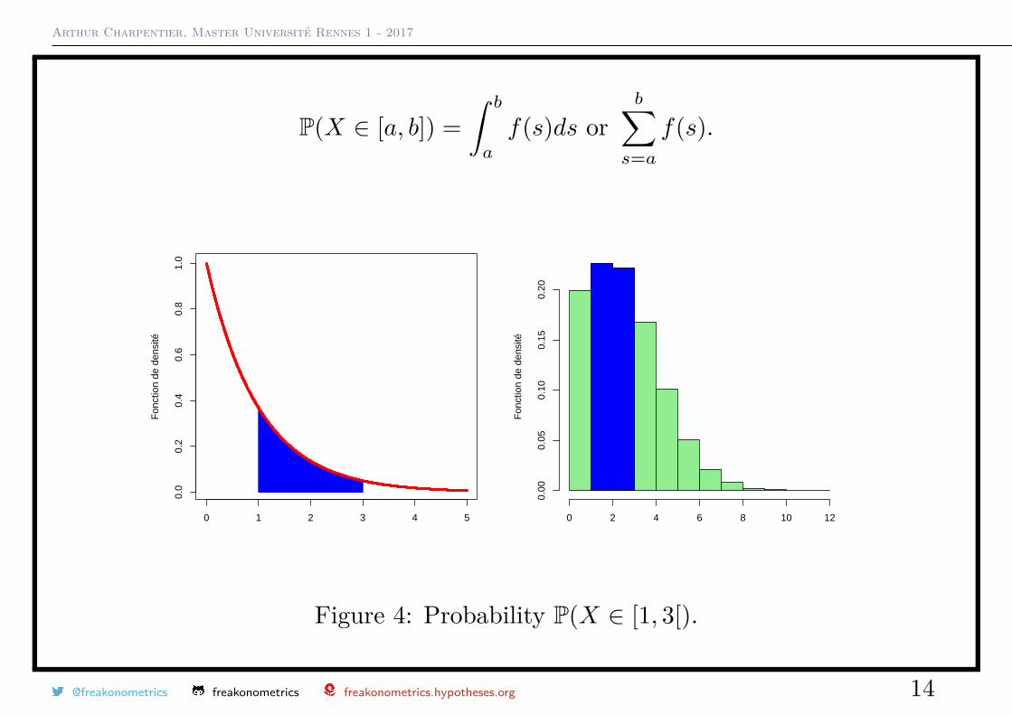
Figure 3: Densities f(x) = F ′(x) or f(x) = P(X = x).
@freakonometrics freakonometrics freakonometrics.hypotheses.org 13
Arthur Charpentier, Master Université Rennes 1 - 2017
P(X ∈ [a, b]) =∫ b
a
f(s)ds orb∑
s=af(s).
0 1 2 3 4 5
0.0
0.2
0.4
0.6
0.8
1.0
Fon
ctio
n de
den
sité
Fon
ctio
n de
den
sité
0 2 4 6 8 10 12
0.00
0.05
0.10
0.15
0.20
Figure 4: Probability P(X ∈ [1, 3[).
@freakonometrics freakonometrics freakonometrics.hypotheses.org 14
Arthur Charpentier, Master Université Rennes 1 - 2017
On Random VectorsDefinition Let Z = (X,Y ) be a random vector. The cumulative distributionfunction of Z is
F (z) = F (x, y) = P(X ≤ x, Y ≤ y), for all z = (x, y) ∈ R× R.
Definition Let Z = (X,Y ) be a random vector. The density of Z is
f(z) = f(x, y) =
∂F (x, y)∂x∂y
in the continuous case, z = (x, y) ∈ R× R
P(X = x, Y = y) in the discrete case, z = (x, y) ∈ N× N
@freakonometrics freakonometrics freakonometrics.hypotheses.org 15
Arthur Charpentier, Master Université Rennes 1 - 2017
On Random VectorsConsider a random vector Z = (X,Y ) with cdf F and density f , one can extractmarginal distributions of X and Y from
FX(x) = P(X ≤ x) = P(X ≤ x, Y ≤ +∞) = limy→∞
F (x, y),
fX(x) = P(X = x) =∞∑y=0
P(X = x, Y = y) =∞∑y=0
f(x, y), for a discrete distribution
fX(x) =∫ ∞−∞
f(x, y)dy for a continuous distribution
@freakonometrics freakonometrics freakonometrics.hypotheses.org 16
Arthur Charpentier, Master Université Rennes 1 - 2017
Conditional distribution Y |XDefine the conditionnal distribution of Y given X = x, with density given byBayes formula
P(Y = y|X = x) = P(X = x, Y = y)P(X = x) in the discrete case,
fY |X=x(y) = f(x, y)fX(x) , in the continuous case.
One can also derive the conditional cdf
P(Y ≤ y|X = x) =y∑t=0
P(Y = t|X = x) =y∑t=0
P(X = x, Y = t)P(X = x) in the discrete case,
FY |X=x(y) =∫ x
−∞fY |X=x(t)dt = 1
fX(x)
∫ x
−∞f(x, t)dt, in the continuous case.
@freakonometrics freakonometrics freakonometrics.hypotheses.org 17
Arthur Charpentier, Master Université Rennes 1 - 2017
On Margins of Random VectorsWe have seen that
fY (y) =∞∑x=0
f(x, y) or∫ ∞−∞
f(x, y)dx
Let us focus on the continuous case.
From Bayes formula,f(x, y) = fY |X=x(y) · fX(x)
and we can writefY (y) =
∫ ∞−∞
fY |X=x(y) · fX(x)dx,
known as the law of total probability.
@freakonometrics freakonometrics freakonometrics.hypotheses.org 18
Arthur Charpentier, Master Université Rennes 1 - 2017
IndependenceDefinition Consider two random variables X and Y . X and Y are independentif one of the following statements is valid
• F (x, y) = FX(x)FY (y) ∀x, y, or P(X ≤ x, Y ≤ y) = P(X ≤ x)× P(Y ≤ y),• f(x, y) = fX(x)fY (y) ∀x, y, or P(X = x, Y = y) = P(X = x)× P(Y = y),• FY |X=x(y) = FY (y) ∀x, y, or fY |X=x(y) = fY (y),• FX|Y=y(y) = FX(x) ∀x, y, or fX|Y=y(y) = fX(x).
We will use notations X ⊥⊥ Y when variables are independent.
@freakonometrics freakonometrics freakonometrics.hypotheses.org 19
Arthur Charpentier, Master Université Rennes 1 - 2017
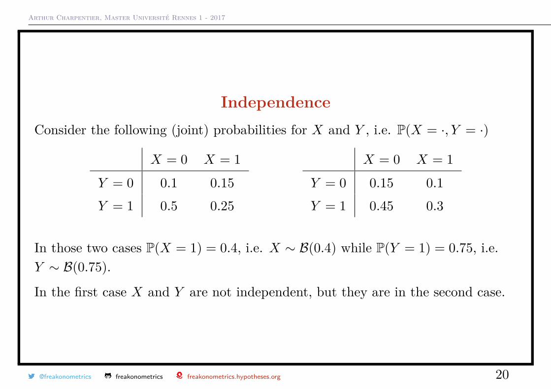
IndependenceConsider the following (joint) probabilities for X and Y , i.e. P(X = ·, Y = ·)
X = 0 X = 1
Y = 0 0.1 0.15Y = 1 0.5 0.25
oooX = 0 X = 1
Y = 0 0.15 0.1Y = 1 0.45 0.3
In those two cases P(X = 1) = 0.4, i.e. X ∼ B(0.4) while P(Y = 1) = 0.75, i.e.Y ∼ B(0.75).
In the first case X and Y are not independent, but they are in the second case.
@freakonometrics freakonometrics freakonometrics.hypotheses.org 20
Arthur Charpentier, Master Université Rennes 1 - 2017
Conditional IndependenceTwo variables X and Y are conditionnally independent given Z if for all z (suchthat P(Z = z) > 0)
P(X ≤ x, Y ≤ y | Z = z) = P(X ≤ x | Z = z) · P(Y ≤ y | Z = z)
For instance, let Z ∈ [0, 1], and consider X|Z = z ∼ B(z) and Y |Z = z ∼ B(z)independent (given Z). Variables are conditionally independent, but notindependent.
@freakonometrics freakonometrics freakonometrics.hypotheses.org 21
Arthur Charpentier, Master Université Rennes 1 - 2017
Moments of a distributionDefinition Let X be a random variable. Its expected value is
E(X) =∫ ∞−∞
x · f(x)dx or∞∑x=0
x · P(X = x)
Definition Let Z = (X,Y ) de random vector. Its expected value is
E(Z) =
E(X)E(Y )
Proposition. The expected value of Y = g(X), where X has density f , is
E(g(X)) =∫ +∞
−∞g(x) · f(x)dx.
If g is nonlinear E(g(X)) 6= g(E(X)).
@freakonometrics freakonometrics freakonometrics.hypotheses.org 22
Arthur Charpentier, Master Université Rennes 1 - 2017
On the expected valueProposition. Let X and Y two random variables with finite expected value
E(αX + βY ) = αE(X) + βE(Y ), ∀α, β, i.e. the expected vallue is linear E(XY ) 6= E(X) · E(Y ) in general, but if X ⊥⊥ Y , equality holds.
The expected value of any random variable is a number in R.
Consider a uniform distribution on [a, b], with density f(x) = 1b− a
1(x ∈ [a, b]),
E(X) =∫Rxf(x)dx = 1
b− a
∫ b
a
xdx = 1b− a
[x2
2
]ba
= 1b− a
b2 − a2
2 = 1b− a
(b− a)(a+ b)2 = a+ b
2 .
@freakonometrics freakonometrics freakonometrics.hypotheses.org 23
Arthur Charpentier, Master Université Rennes 1 - 2017
If E[|X|] <∞, we note X ∈ L1.
There are cases where expected value is infinite (does not exist)
Consider a repeated head/tail game, where gains are double when ‘head’ isobtained, and we can play again, until we get a ‘tail’
E(X) = 1× P(‘tail’ at 1st draw)+1× 2× P(‘tail’ at 2nd draw)+2× 2× P(‘tail’ at 3rd draw)+4× 2× P(‘tail’ at 4th draw)+8× 2× P(‘tail’ at 5th draw) + · · ·
= 12 + 2
4 + 48 + 8
16 + 1632 + 32
64 + · · · =∞.
(so called St Petersburg paradox)
@freakonometrics freakonometrics freakonometrics.hypotheses.org 24
Arthur Charpentier, Master Université Rennes 1 - 2017
Conditional ExpectationDefinition Let X and Y be two random variables. The conditional expectationof Y given X = x is the expected value of the conditional distribution Y |X = x,
E(Y |X = x) =∫ ∞−∞
y · fY |X=x(y)dy ou∞∑x=0
y · P(Y = y|X = x).
E(Y |X = x) is a function of x, E(Y |X = x) = ϕ(x). Random variable ϕ(X)might be denoted E(Y |X).Proposition. E(Y |X) being a random variable, observe that
E[E(Y |X)
]= E(Y )
@freakonometrics freakonometrics freakonometrics.hypotheses.org 25
Arthur Charpentier, Master Université Rennes 1 - 2017
Proof.
E (E(X|Y )) =∑y
E(X|Y = y) · P(Y = y)
=∑y
(∑x
x · P(X = x|Y = y))· P(Y = y)
=∑y
∑x
x · P(X = x|Y = y) · P(Y = y)
=∑x
∑y
x · P(Y = y|X = x) · P(X = x)
=∑x
x · P(X = x) ·(∑
y
P(Y = y|X = x))
=∑x
x · P(X = x) = E(X).
@freakonometrics freakonometrics freakonometrics.hypotheses.org 26
Arthur Charpentier, Master Université Rennes 1 - 2017
Higher Order MomentsBefore introducting the order 2 moment, recall that
E(g(X)) =∫ +∞
−∞g(x) · f(x)dx
E(g(X,Y )) =∫ +∞
−∞
∫ +∞
−∞g(x, y) · f(x, y)dxdy.
Definition Let X be a random variable. The variance of X is
Var(X) = E[(X−E(X))2] =∫ ∞−∞
(x−E(X))2·f(x)dx or∞∑x=0
(x−E(X))2·P(X = x).
Equivalently Var(X) = E[X2]− (E[X])2
The variance measures the dispersion of X around E(X), and it is a positivenumber.
√Var(X) is called the standard deviation.
@freakonometrics freakonometrics freakonometrics.hypotheses.org 27
Arthur Charpentier, Master Université Rennes 1 - 2017
Higher Order MomentsDefinition Let Z = (X,Y ) be a random vector. The variance-covariance matrixof Z is
Var(Z) =
Var(X) Cov(X,Y )Cov(Y,X) Var(Y )
where Var(X) = E[(X − E(X))2] and
Cov(X,Y ) = E[(X − E(X)) · (Y − E(Y ))] = Cov(Y,X).
Definition Let Z = (X,Y ) be a random vector. The (Pearson) correlationbetween X and Y is
corr(X,Y ) = Cov(X,Y )√Var(X) ·Var(Y )
= E[(X − E(X)) · (Y − E(Y ))]√E[(X − E(X))]2 · E[(Y − E(Y ))]2
.
@freakonometrics freakonometrics freakonometrics.hypotheses.org 28
Arthur Charpentier, Master Université Rennes 1 - 2017
On the VarianceProposition. The variance is always positive, and Var(X) = 0 if and only if Xis a constant.Proposition. The variance is not linear, but
Var(αX + βY ) = α2Var(X) + 2αβCov(X,Y ) + β2Var(Y ).
A consequence is that
Var(
n∑i=1
Xi
)=
n∑i=1
Var (Xi)+∑j 6=i
Cov(Xi, Xj) =n∑i=1
Var (Xi)+2∑j>i
Cov(Xi, Xj).
Proposition. Variance is (usually) nonlinear, but Var(α+ βX) = β2Var(X).
If Var[X] <∞ - or E[X2] <∞ - we note X ∈ L2.
@freakonometrics freakonometrics freakonometrics.hypotheses.org 29
Arthur Charpentier, Master Université Rennes 1 - 2017
On covarianceProposition. Consider random variables X, X1, X2 and Y , then
• Cov(X,Y ) = E(XY )− E(X)E(Y ),• Cov(αX1 + βX2, Y ) = αCov(X1, Y ) + βCov(X2, Y ).
Cov(X,Y ) =∑ω∈Ω
[X(ω)− E(X)] · [Y (ω)− E(Y )] · P(ω)
Heuristically, a positive covariance should mean that for a majority of events ω,the following inequality should hold
[X(ω)− E(X)] · [Y (ω)− E(Y )] ≥ 0.
X(ω) ≥ E(X) and Y (ω) ≥ E(Y ), i.e. X and Y take together large values X(ω) ≤ E(X) and Y (ω) ≤ E(Y ), i.e. X and Y take together small values
Proposition. If X and Y are independent, (X ⊥⊥ Y ), then Cov(X,Y ) = 0, butthe converse is usually false.
@freakonometrics freakonometrics freakonometrics.hypotheses.org 30
Arthur Charpentier, Master Université Rennes 1 - 2017
Conditionnal VarianceDefinition Let X and Y be two random variables. The conditional variance ofY given X = x is the variance of the conditional distribution Y |X = x,
Var(Y |X = x) =∫ ∞−∞
[y − E(Y |X = x)]2 · fY |X=x(y)dy.
Var(Y |X = x) is a function of x, Var(Y |X = x) = ψ(x). Random variable ψ(X)will be denoted Var(Y |X).Proposition. Var(Y |X) being a random variable,
Var(Y ) = Var[E(Y |X)] + E[Var(Y |X)],
which is the variance decomposition formula.
@freakonometrics freakonometrics freakonometrics.hypotheses.org 31
Arthur Charpentier, Master Université Rennes 1 - 2017
Conditionnal Variance
Proof. Use the following decomposition
Var(Y ) = E[(Y − E(Y ))2] = E[(Y−E(Y |X) + E(Y |X)− E(Y ))2]= E[([Y − E(Y |X)] + [E(Y |X)− E(Y )])2]= E[([Y − E(Y |X)])2] + E[([E(Y |X)− E(Y )])2]
+2E[[Y − E(Y |X)] · [E(Y |X)− E(Y )]]
Then observe that
E[([Y − E(Y |X)])2] = E(E((Y − E(Y |X))2|X)
)= E[ Var(Y |X)],
E[([E(Y |X)− E(Y )])2] = E[([E(Y |X)− E(E(Y |X))])2] = Var[E(Y |X)].
The expected value of the cross-product is null (given X).
@freakonometrics freakonometrics freakonometrics.hypotheses.org 32
Arthur Charpentier, Master Université Rennes 1 - 2017
Geometric PerspectiveRecall that L2 is the set of random variables with finite variance
• < X,Y >= E(XY ) is a scalar product• ‖X‖ =
√E(X2) is a norm (denoted ‖ · ‖2).
E(X) is the orthogonal projection of X on the set of constants
E(X) = argmina∈R‖X − a‖2 = E([X − a]2).
The correlation is the cosinus of the angle between X − E(X) and Y − E(Y ): ifCorr(X,Y ) = 0 variables are orthogonal, X ⊥ Y (weaker than X ⊥⊥ Y ).
If L2X is the set of random variables generated from X (that can be written
ϕ(X)) with finite variance. E(Y |X) is the orthogonal projection of Y on L2X
E(Y |X) = argminϕ‖Y − ϕ(X)‖2 = E([Y − ϕ(X)]2).
E(Y |X) is the best approximation of Y by a function of X.
@freakonometrics freakonometrics freakonometrics.hypotheses.org 33
Arthur Charpentier, Master Université Rennes 1 - 2017
Conditional ExpectationIn an econometric model, we want to ‘explain’ Y by X.
linear econometrics, E(Y |X) ∼ EL(Y |X) = β0 + β1X. nonlinear econometrics, E(Y |X) = ϕ(X).
or more generally, ‘explain’ Y by X.
linear econometrics, E(Y |X) ∼ EL(Y |X) = β0 + β1X1 + · · ·+ βkXk. nonlinear econometrics, E(Y |X) = ϕ(X) = ϕ(X1, · · · , Xk).
In a time series context, we want to ‘explain’ Xt with Xt−1, Xt−2, · · · .
linear time series,E(Xt|Xt−1, Xt−2, · · · ) ∼ EL(Xt|Xt−1, Xt−2, · · · ) = β0+β1Xt−1+· · ·+βkXt−k
(autoregressive). nonlinear time series, E(Xt|Xt−1, Xt−2, · · · ) = ϕ(Xt−1, Xt−2, · · · ).
@freakonometrics freakonometrics freakonometrics.hypotheses.org 34
Arthur Charpentier, Master Université Rennes 1 - 2017
Sum of Random VariablesProposition. Let X and Y be two discrete random variables, then thedistribution of S = X + Y is
P(S = s) =∞∑
k=−∞P(X = k)× P(Y = s− k).
Let X and Y be two (abs) continuous random variables, then the distribution ofS = X + Y is
fS(s) =∫ ∞−∞
fX(x)× fY (s− x)dx.
Note fS = fX ? fY where ? is the convolution operator.
@freakonometrics freakonometrics freakonometrics.hypotheses.org 35
Arthur Charpentier, Master Université Rennes 1 - 2017
More on the Moments of a Distributionn-th order moment of a random variable X is µn = E[Xn], if that value is finite.Let µ′n denote centered moments.
Some of those moments :
• Order 1 moment µ = E[X] is the expected value• Centered order 2 moment: µ′2 = E
[(X − µ)2
]is the variance, σ2.
• Centered and Reduced order 3 moment: µ′3 = E
[(X − µσ
)3]is an
assymmetric coefficient, called skewness.
• Centered and Reduced order 4 moment: µ′4 = E
[(X − µσ
)4]is called
kurtosis.
@freakonometrics freakonometrics freakonometrics.hypotheses.org 36
Arthur Charpentier, Master Université Rennes 1 - 2017
Some Probabilistic Distributions: BernoulliThe Bernoulli distribution B(p), p ∈ (0, 1)
P(X = 0) = 1− p and P(X = 1) = p.
Then E(X) = p and Var(X) = p(1− p).
@freakonometrics freakonometrics freakonometrics.hypotheses.org 37
Arthur Charpentier, Master Université Rennes 1 - 2017
Some Probabilistic Distributions: BinomialThe Binomial distribution B(n, p), p ∈ (0, 1) and n ∈ N∗
P(X = k) =(n
k
)pk(1− p)n−k where k = 0, 1, · · · , n,
(n
k
)= n!k!(n− k)!
Then E(X) = np and Var(X) = np(1− p).
If X1, · · · , Xn ∼ B(p) are independent, then X = X1 + · · ·+Xn ∼ B(n, p).
With R, dbinom(x, size, prob), qbinom() and pbinom() are respectively the cdf, thequantile function and the probability function of B(n, p) where n is the size andp the prob parameter.
@freakonometrics freakonometrics freakonometrics.hypotheses.org 38
Arthur Charpentier, Master Université Rennes 1 - 2017
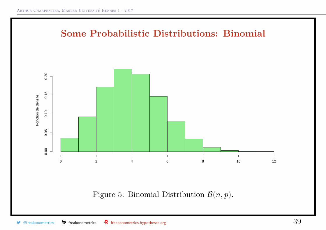
Some Probabilistic Distributions: BinomialF
onct
ion
de d
ensi
té
0 2 4 6 8 10 12
0.00
0.05
0.10
0.15
0.20
Figure 5: Binomial Distribution B(n, p).
@freakonometrics freakonometrics freakonometrics.hypotheses.org 39
Arthur Charpentier, Master Université Rennes 1 - 2017
Some Probabilistic Distributions: PoissonThe Poisson distribution P(λ), λ > 0
P(X = k) = exp(−λ)λk
k! where k = 0, 1, · · ·
Then E(X) = λ and Var(X) = λ.
Further, if X1 ∼ P(λ1) and X2 ∼ P(λ2) are independent, then
X1 +X2 ∼ P(λ1 + λ2)
Observe that a recursive equation can be obtained
P (X = k + 1)P (X = k) = λ
k + 1 pour k ≥ 1
With R, dpois(x, lambda), qpois() and ppois() are respectively the probabilityfunction, the quantile function and the cdf.
@freakonometrics freakonometrics freakonometrics.hypotheses.org 40
Arthur Charpentier, Master Université Rennes 1 - 2017
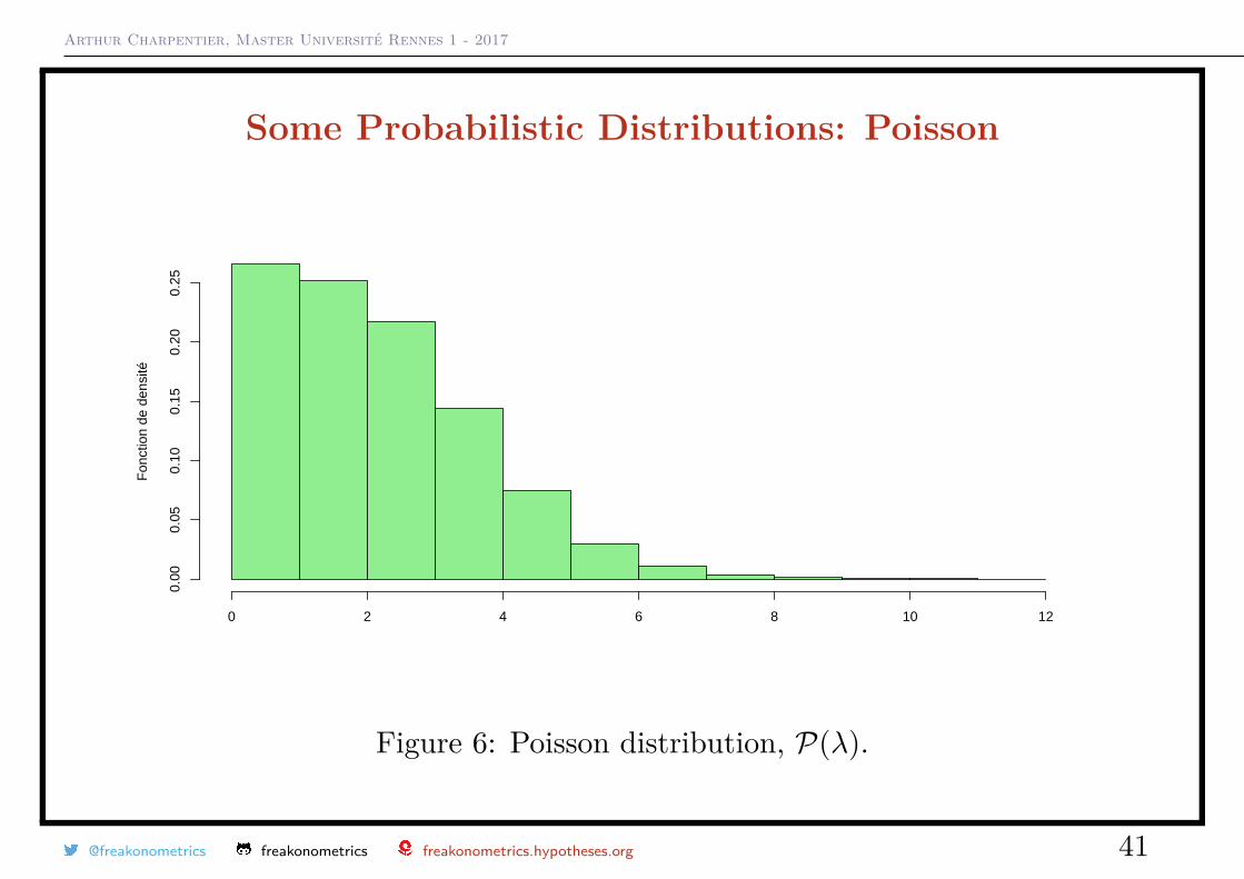
Some Probabilistic Distributions: PoissonF
onct
ion
de d
ensi
té
0 2 4 6 8 10 12
0.00
0.05
0.10
0.15
0.20
0.25
Figure 6: Poisson distribution, P(λ).
@freakonometrics freakonometrics freakonometrics.hypotheses.org 41
Arthur Charpentier, Master Université Rennes 1 - 2017
Some Probabilistic Distributions: GeometricThe Geometrica G(p), p ∈]0, 1[
P (X = k) = p (1− p)k−1 for k = 1, 2, · · ·
with cdf P (N ≤ k) = 1− pk.
Observe that this distribution satisfies the following relationship
P (X = k + 1)P (X = k) = 1− p (= constant) for k ≥ 1
First moments are here
E (X) = 1pand Var (X) = 1− p
p2 .
aIt is also possible to define such a distribution on N, instead of N\ 0.
@freakonometrics freakonometrics freakonometrics.hypotheses.org 42
Arthur Charpentier, Master Université Rennes 1 - 2017
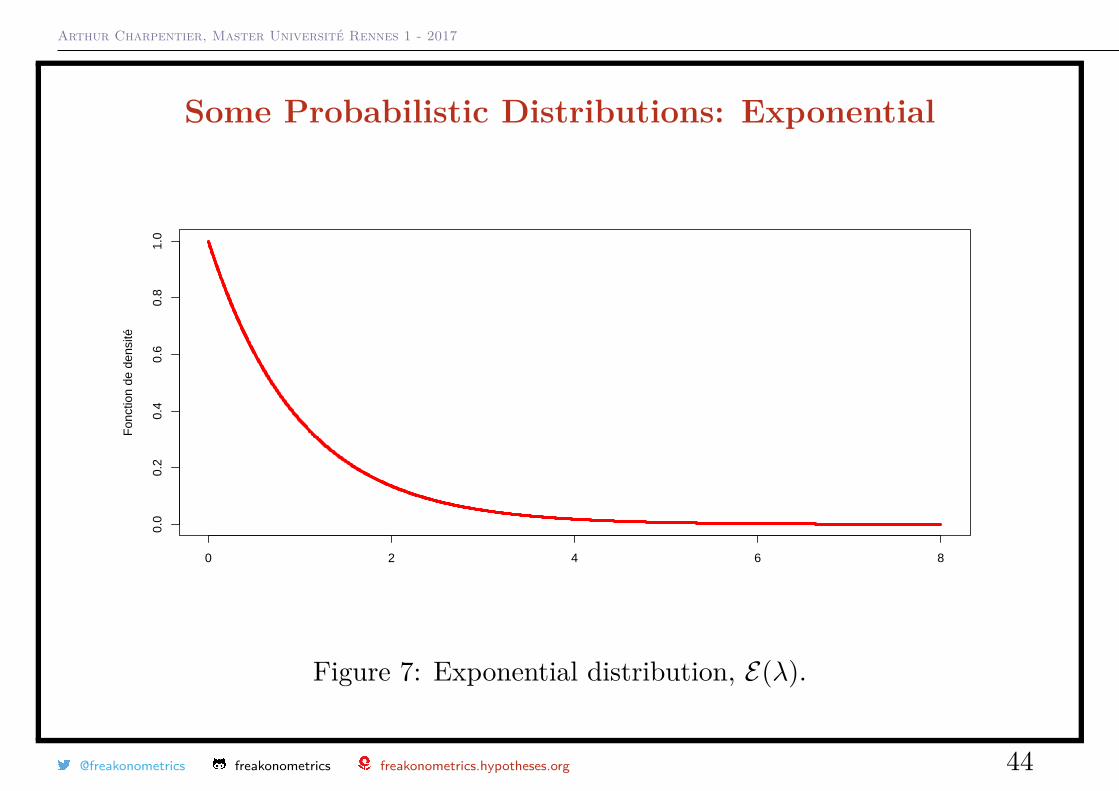
Some Probabilistic Distributions: ExponentialThe exponential distribution E(λ), with λ > 0
F (x) = P(X ≤ x) = e−λx where x ≥ 0, f(x) = λe−λx.
Then E(X) = 1/λ and Var(X) = 1/λ2.
This is a memoryless distribution, since
P(X > x+ t|X > x) = P(X > t).
In R, dexp(x, rate), qexp() and pexp() are respectively the cdf, the quantilefunction and the density.
@freakonometrics freakonometrics freakonometrics.hypotheses.org 43
Arthur Charpentier, Master Université Rennes 1 - 2017
Some Probabilistic Distributions: Exponential
0 2 4 6 8
0.0
0.2
0.4
0.6
0.8
1.0
Fon
ctio
n de
den
sité
Figure 7: Exponential distribution, E(λ).
@freakonometrics freakonometrics freakonometrics.hypotheses.org 44
Arthur Charpentier, Master Université Rennes 1 - 2017
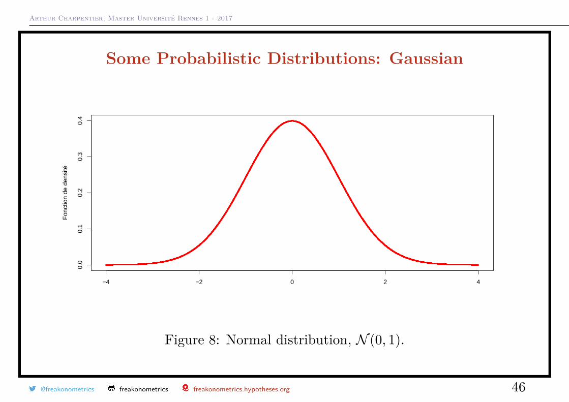
Some Probabilistic Distributions: GaussianThe Gaussian (or normal) distribution N (µ, σ2), with µ ∈ R and σ > 0
f(x) = 1√2πσ2
exp(− (x− µ)2
2σ2
), for all x ∈ R.
Then E(X) = µ and Var(X) = σ2.
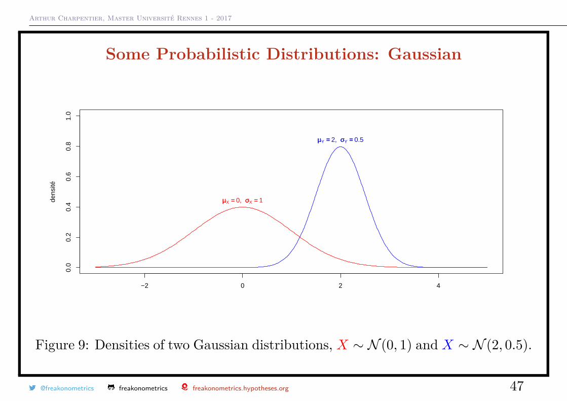
Observe that if Z ∼ N (0, 1), X = µ+ σZ ∼ N (µ, σ2).
With R, dnorm(x, mean, sd), qnorm() and pnorm() are respectively the cumulativedistribution function, the quantile function and the density.
With R, dnorm(x,mean=a,sd=b) for the N (a, b) density.
@freakonometrics freakonometrics freakonometrics.hypotheses.org 45
Arthur Charpentier, Master Université Rennes 1 - 2017
Some Probabilistic Distributions: Gaussian
−4 −2 0 2 4
0.0
0.1
0.2
0.3
0.4
Fon
ctio
n de
den
sité
Figure 8: Normal distribution, N (0, 1).
@freakonometrics freakonometrics freakonometrics.hypotheses.org 46
Arthur Charpentier, Master Université Rennes 1 - 2017
Some Probabilistic Distributions: Gaussian
−2 0 2 4
0.0
0.2
0.4
0.6
0.8
1.0
dens
ité
µµX == 0, σσX == 1
µµY == 2, σσY == 0.5
Figure 9: Densities of two Gaussian distributions, X ∼ N (0, 1) and X ∼ N (2, 0.5).
@freakonometrics freakonometrics freakonometrics.hypotheses.org 47
Arthur Charpentier, Master Université Rennes 1 - 2017
Probability DistributionsThe Gaussian vector N (µ,Σ) : X = (X1, ..., Xn) is a Gaussian vector withmean E (X) = µ and covariance matrix Σ = E
((X − µ) (X − µ)T
)non-degenerated (Σ est invertible) if its density is
f (x) = 1(2π)n/2
√det Σ
exp(−1
2 (x− µ)T Σ−1 (x− µ)), x ∈ Rd,
Proposition. Let X = (X1, ..., Xn) be a random vector with values in Rd, thenX is a Gaussian vector if and only if for any a = (a1, ..., an) ∈ Rd,aTX = a1X1 + ...+ anXn has a (univariate) Gaussian distribution.
@freakonometrics freakonometrics freakonometrics.hypotheses.org 48
Arthur Charpentier, Master Université Rennes 1 - 2017
Probability DistributionsHence, if X is a Gaussian vector, then for any i, Xi has a (univariate) Gaussiandistribution, but its converse it not necessarily true.Proposition. Let X = (X1, ..., Xn) be a random vector with mean E (X) = µ
and with covariance matrix Σ, if A is a k × n matrix, and b ∈ Rk, thenY = AX + b is a Gaussian vector Rk, with distribution N
(Aµ,AΣAT
).
For example, in a regression model, y = Xβ + ε, where ε ∼ N (0, σ2I), the OLSestimator of β is β = [XTX]−1XTy can be written
β = [XTX]−1XT(Xβ + ε) = β +XTX]−1XT︸ ︷︷ ︸A
ε︸︷︷︸∼N (0,σ2I)
∼ N (β, σ2[XTX]−1)
Observe that if (X1, X2) is a Gaussian vector X1 and X2 are independent if andonly if
Cov (X1, X2) = E ((X1 − E (X1)) (X2 − E (X2))) = 0.
@freakonometrics freakonometrics freakonometrics.hypotheses.org 49
Arthur Charpentier, Master Université Rennes 1 - 2017
Probability DistributionsProposition. If X = (X1,X2) is a Gaussian vector with mean
E (X) = µ =
µ1
µ2
and covariance matrix covariance Σ =
Σ11 Σ12
Σ21 Σ22
, thenX2|X1 = x1 ∼ N
(µ1 + Σ12Σ−1
22 (x1 − µ2) ,Σ11 − Σ12Σ−122 Σ21
).
Cf autoregressive time series Xt = ρXt−1 + εt, where X0 = 0, ε1, · · · , εn i.i.d.N (0, σ2), i.e. ε = (ε1, · · · , εn) ∼ N (0, σ2I). Then
X = (X1, · · · , Xn) ∼ N (0,Σ),Σ = [Σi,j ] = [Cov(Xi, Xj)] = [ρ|i−j|].
@freakonometrics freakonometrics freakonometrics.hypotheses.org 50
Arthur Charpentier, Master Université Rennes 1 - 2017
Probability DistributionIn dimension 2, a vector (X,Y ) centered (i.e. µ = 0) is a Gaussian vector if itsdensity is
f(x, y) = 12πσxσy
√1− ρ2
exp(− 1
2(1− ρ2)
(x2
σ2x
+ y2
σ2y
− 2ρxy(σxσy)
))with covariance matrix Σ is
Σ =
σ2x ρσxσy
ρσxσy σ2y
.
@freakonometrics freakonometrics freakonometrics.hypotheses.org 51
Arthur Charpentier, Master Université Rennes 1 - 2017
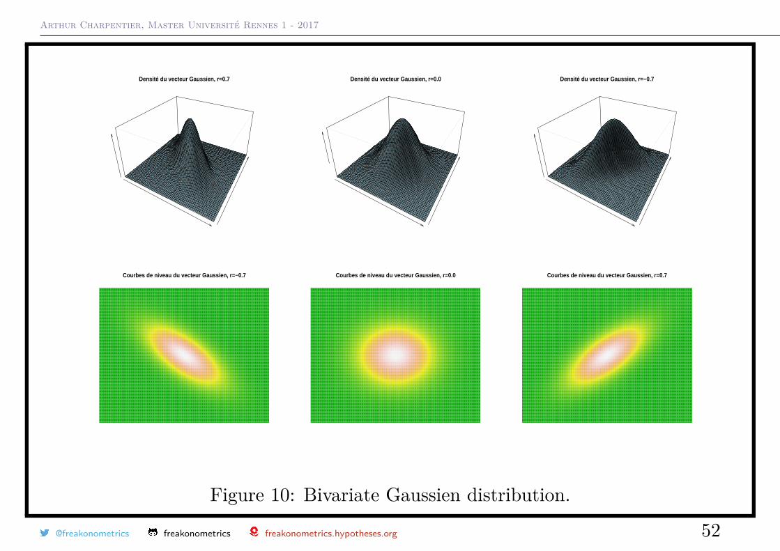
Densité du vecteur Gaussien, r=0.7 Densité du vecteur Gaussien, r=0.0 Densité du vecteur Gaussien, r=−0.7
Courbes de niveau du vecteur Gaussien, r=−0.7 Courbes de niveau du vecteur Gaussien, r=0.0 Courbes de niveau du vecteur Gaussien, r=0.7
Figure 10: Bivariate Gaussien distribution.
@freakonometrics freakonometrics freakonometrics.hypotheses.org 52
Arthur Charpentier, Master Université Rennes 1 - 2017
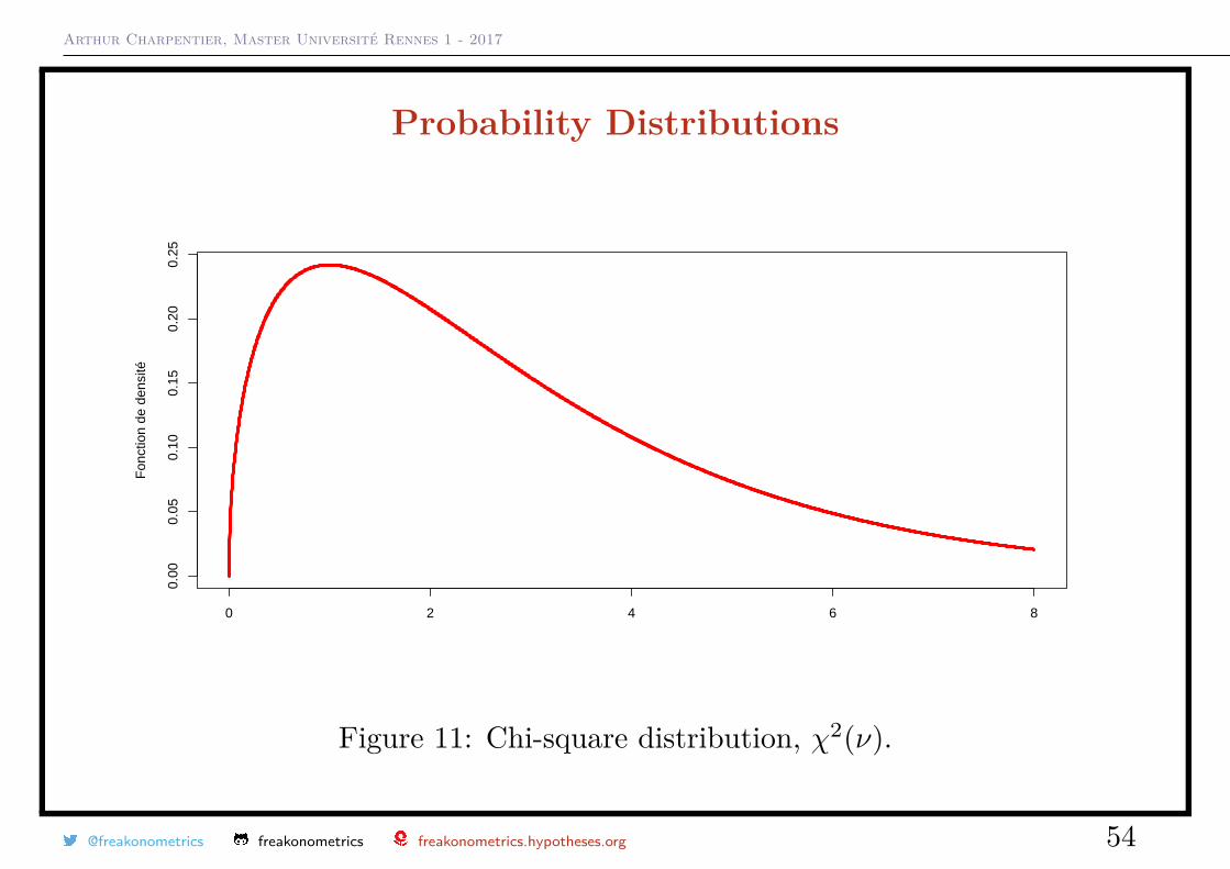
Probability DistributionsThe chi-square distribution χ2(ν), with ν ∈ N∗ has density
x 7→ (1/2)ν/2
Γ(ν/2) xν/2−1e−x/2, where x ∈ [0; +∞[,
where Γ denotes the Gamma function (Γ(n+ 1) = n!). Observe that E(X) = ν etVar(X) = 2ν. ν are the degrees of freedomProposition. If X1, · · · , Xν ∼ N (0, 1) are independent variables, then
Y =ν∑i=1
X2i ∼ χ2(ν), when ν ∈ N.
With R, dchisq(x, df), qchisq() and pchisq() are respectively the cdf, the quantilefunction and the density.
This is a particular case of the Gamma distribution, X ∼ G(k
2 ,12
)
@freakonometrics freakonometrics freakonometrics.hypotheses.org 53
Arthur Charpentier, Master Université Rennes 1 - 2017
Probability Distributions
0 2 4 6 8
0.00
0.05
0.10
0.15
0.20
0.25
Fon
ctio
n de
den
sité
Figure 11: Chi-square distribution, χ2(ν).
@freakonometrics freakonometrics freakonometrics.hypotheses.org 54
Arthur Charpentier, Master Université Rennes 1 - 2017
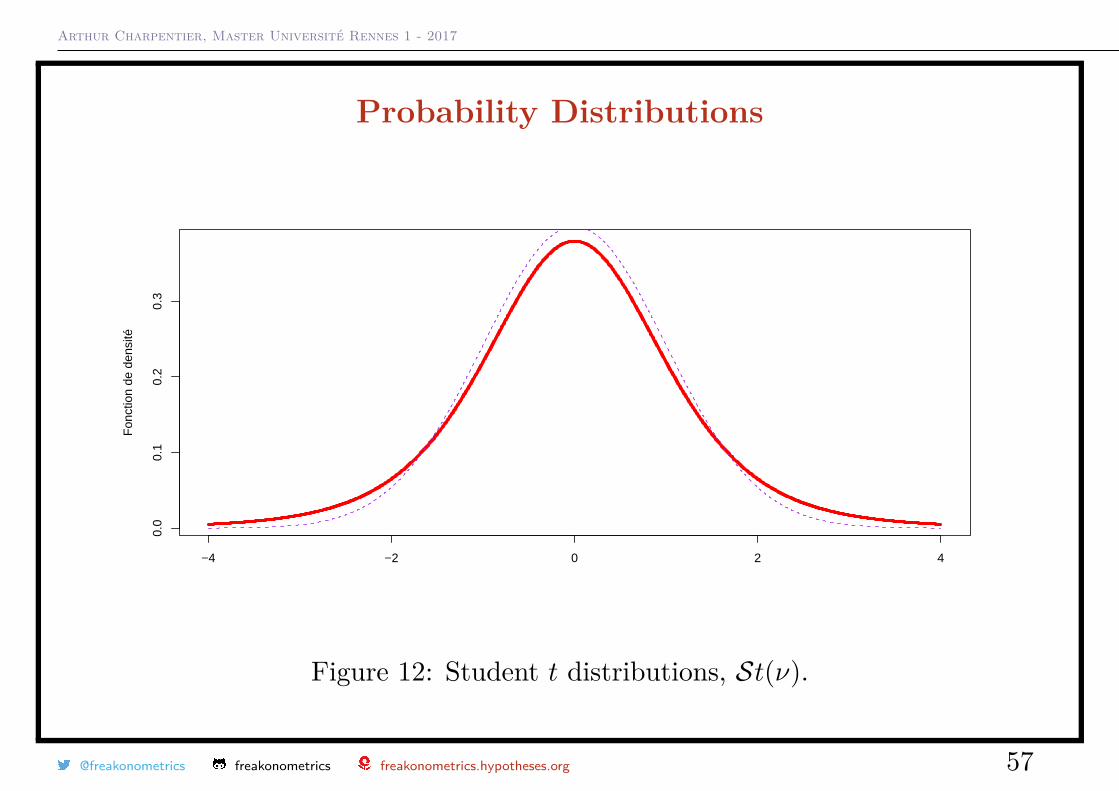
Probability DistributionsThe Student-t distribution St(ν), has density
f(t) =Γ(ν+1
2 )√νπ Γ(ν2 )
(1 + t2
ν
)−( ν+12 )
,
Observe thatE(X) = 0 and Var(X) = ν
ν − 2 when ν > 2.
Proposition. If X ∼ N (0, 1) and Y ∼ χ2(ν) are independents, then
T = X√Y/ν
∼ St(ν).
@freakonometrics freakonometrics freakonometrics.hypotheses.org 55
Arthur Charpentier, Master Université Rennes 1 - 2017
Probability DistributionsLet X1, · · · , Xn be N (µ, σ2) independent random variables. Let
Xn = X1 + · · ·+Xn
nand Sn2 = 1
n− 1
n∑i=1
(Xi −Xn
)2.
Then (n− 1)S2n
σ2 has a χ2(n− 1) distribution, and furthermore
T =√nXn − µSn
∼ St(n− 1).
With R, dt(x, df), qt() and pt() are respectively the cdf, the quantile and thedensity functions.
@freakonometrics freakonometrics freakonometrics.hypotheses.org 56
Arthur Charpentier, Master Université Rennes 1 - 2017
Probability Distributions
−4 −2 0 2 4
0.0
0.1
0.2
0.3
Fon
ctio
n de
den
sité
Figure 12: Student t distributions, St(ν).
@freakonometrics freakonometrics freakonometrics.hypotheses.org 57
Arthur Charpentier, Master Université Rennes 1 - 2017
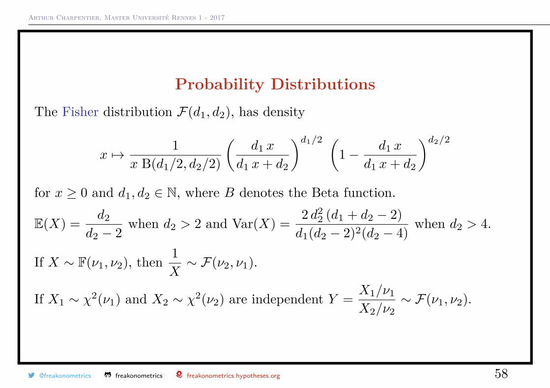
Probability DistributionsThe Fisher distribution F(d1, d2), has density
x 7→ 1x B(d1/2, d2/2)
(d1 x
d1 x+ d2
)d1/2 (1− d1 x
d1 x+ d2
)d2/2
for x ≥ 0 and d1, d2 ∈ N, where B denotes the Beta function.
E(X) = d2
d2 − 2 when d2 > 2 and Var(X) = 2 d22 (d1 + d2 − 2)
d1(d2 − 2)2(d2 − 4) when d2 > 4.
If X ∼ F(ν1, ν2), then 1X∼ F(ν2, ν1).
If X1 ∼ χ2(ν1) and X2 ∼ χ2(ν2) are independent Y = X1/ν1
X2/ν2∼ F(ν1, ν2).
@freakonometrics freakonometrics freakonometrics.hypotheses.org 58
Arthur Charpentier, Master Université Rennes 1 - 2017
Probability DistributionsWith R, df(x, df1, df2), qf() and pf() denote the cdf, the quantile and thedensity functions.
@freakonometrics freakonometrics freakonometrics.hypotheses.org 59
Arthur Charpentier, Master Université Rennes 1 - 2017
0 2 4 6 8
0.0
0.1
0.2
0.3
0.4
0.5
0.6
0.7
Fon
ctio
n de
den
sité
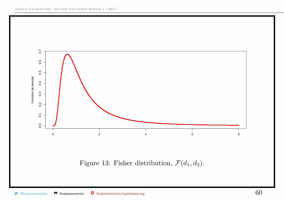
Figure 13: Fisher distribution, F(d1, d2).
@freakonometrics freakonometrics freakonometrics.hypotheses.org 60
Arthur Charpentier, Master Université Rennes 1 - 2017
Conditional Distributions
• Mixture of Bernoulli distribution B(Θ)
Let Θ denote a random variable taking values θ1, θ2 ∈ [0, 1] with probabilities p1
and p2 (with p1 + p2 = 1). Assume that
X|Θ = θ1 ∼ B(θ1) and X|Θ = θ2 ∼ B(θ2).
The non-conditionnal distribution of X is
P(X = x) =∑θ
P(X = x|Θ = θ)·P(Θ = θ) = P(X = x|Θ = θ1)·p1+P(X = x|Θ = θ2)·p2,
P(X = 0) = P(X = 0|Θ = θ1) · p1 + P(X = 0|Θ = θ2) · p2 = 1− θ1p1 − θ2p2
P(X = 1) = P(X = 1|Θ = θ1) · p1 + P(X = 1|Θ = θ2) · p2 = θ1p1 + θ2p2
i.e. X ∼ B(θ1p1 + θ2p2).
@freakonometrics freakonometrics freakonometrics.hypotheses.org 61
Arthur Charpentier, Master Université Rennes 1 - 2017
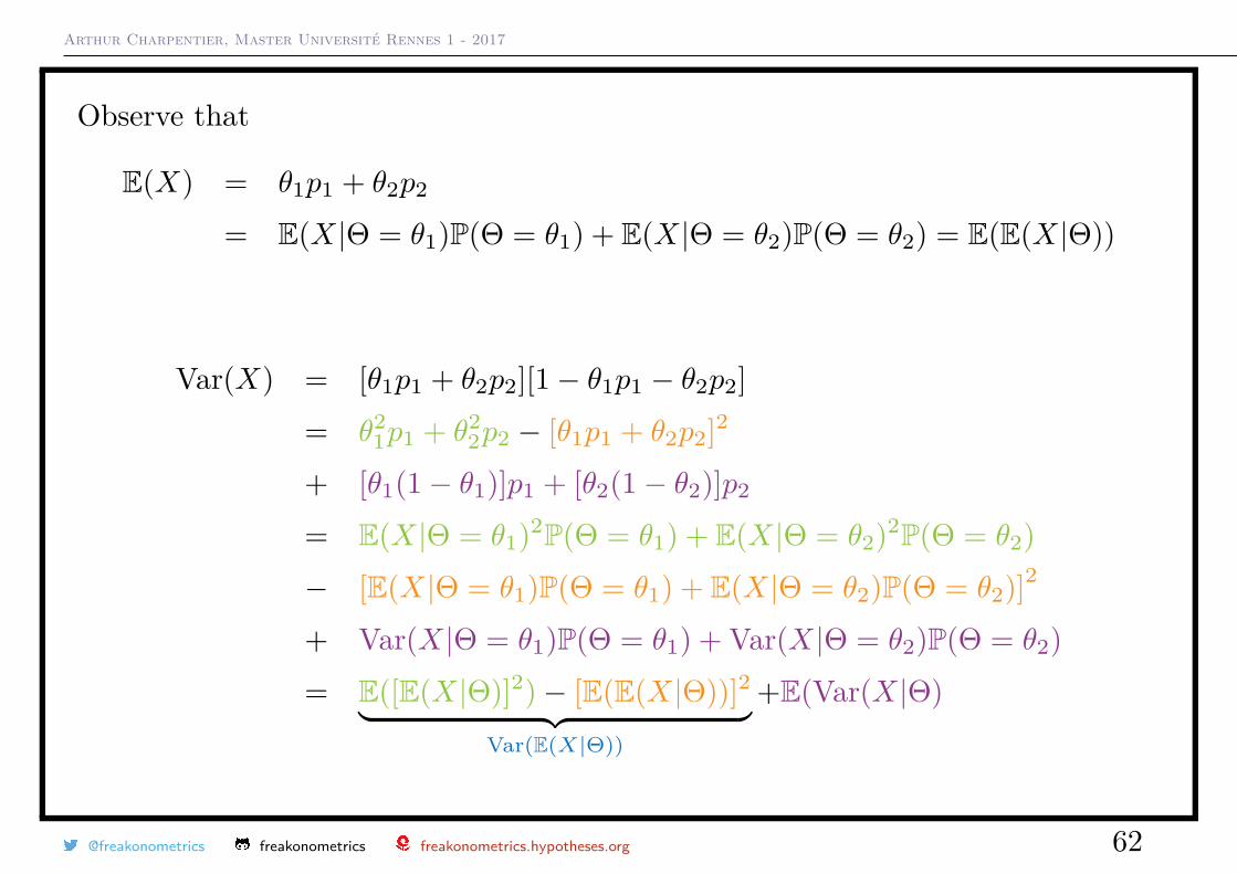
Observe that
E(X) = θ1p1 + θ2p2
= E(X|Θ = θ1)P(Θ = θ1) + E(X|Θ = θ2)P(Θ = θ2) = E(E(X|Θ))
Var(X) = [θ1p1 + θ2p2][1− θ1p1 − θ2p2]= θ2
1p1 + θ22p2 − [θ1p1 + θ2p2]2
+ [θ1(1− θ1)]p1 + [θ2(1− θ2)]p2
= E(X|Θ = θ1)2P(Θ = θ1) + E(X|Θ = θ2)2P(Θ = θ2)− [E(X|Θ = θ1)P(Θ = θ1) + E(X|Θ = θ2)P(Θ = θ2)]2
+ Var(X|Θ = θ1)P(Θ = θ1) + Var(X|Θ = θ2)P(Θ = θ2)= E([E(X|Θ)]2)− [E(E(X|Θ))]2︸ ︷︷ ︸
Var(E(X|Θ))
+E(Var(X|Θ)
@freakonometrics freakonometrics freakonometrics.hypotheses.org 62
Arthur Charpentier, Master Université Rennes 1 - 2017
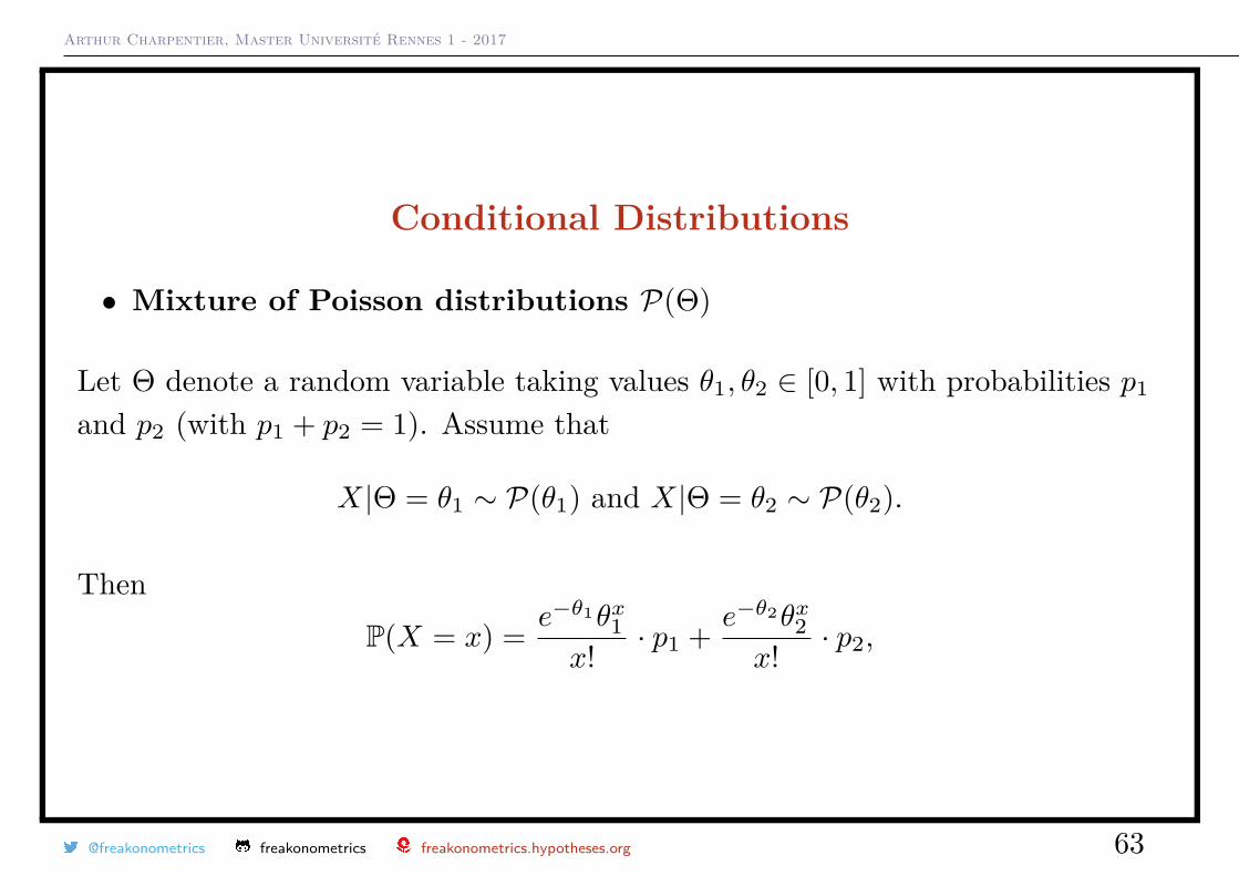
Conditional Distributions
• Mixture of Poisson distributions P(Θ)
Let Θ denote a random variable taking values θ1, θ2 ∈ [0, 1] with probabilities p1
and p2 (with p1 + p2 = 1). Assume that
X|Θ = θ1 ∼ P(θ1) and X|Θ = θ2 ∼ P(θ2).
ThenP(X = x) = e−θ1θx1
x! · p1 + e−θ2θx2x! · p2,
@freakonometrics freakonometrics freakonometrics.hypotheses.org 63
Arthur Charpentier, Master Université Rennes 1 - 2017
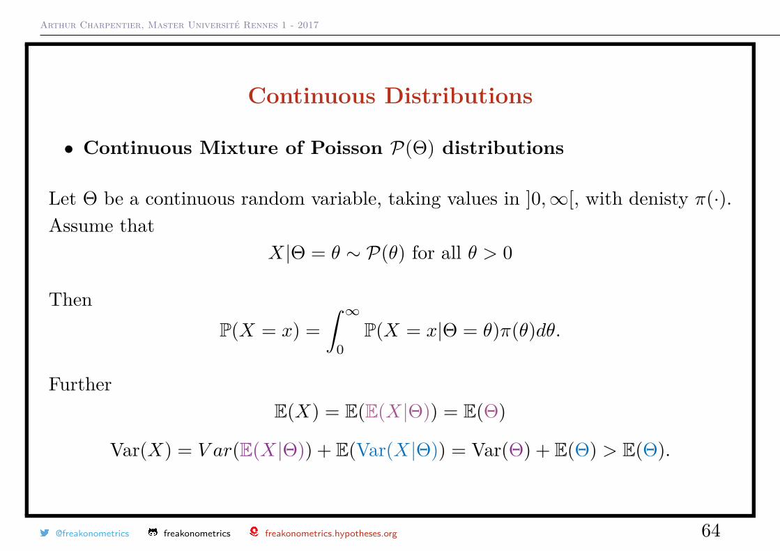
Continuous Distributions
• Continuous Mixture of Poisson P(Θ) distributions
Let Θ be a continuous random variable, taking values in ]0,∞[, with denisty π(·).Assume that
X|Θ = θ ∼ P(θ) for all θ > 0
ThenP(X = x) =
∫ ∞0
P(X = x|Θ = θ)π(θ)dθ.
FurtherE(X) = E(E(X|Θ)) = E(Θ)
Var(X) = V ar(E(X|Θ)) + E(Var(X|Θ)) = Var(Θ) + E(Θ) > E(Θ).
@freakonometrics freakonometrics freakonometrics.hypotheses.org 64
Arthur Charpentier, Master Université Rennes 1 - 2017
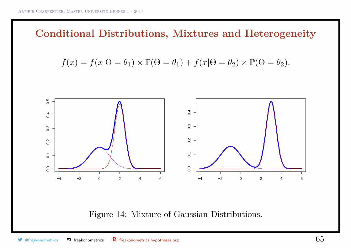
Conditional Distributions, Mixtures and Heterogeneity
f(x) = f(x|Θ = θ1)× P(Θ = θ1) + f(x|Θ = θ2)× P(Θ = θ2).
−4 −2 0 2 4 6
0.0
0.1
0.2
0.3
0.4
0.5
−4 −2 0 2 4 6
0.0
0.1
0.2
0.3
0.4
Figure 14: Mixture of Gaussian Distributions.
@freakonometrics freakonometrics freakonometrics.hypotheses.org 65
Arthur Charpentier, Master Université Rennes 1 - 2017
Conditional Distributions, Mixtures and HeterogeneityMixtures are related to heterogeneity.
In linear econometric models, Y |X = x ∼ N (xTβ, σ2).
In logit/probit models, Y |X = x ∼ B(p[xTβ]) where p[xTβ] = exTβ
1 + exTβ.
E.g. Y |X1 = male ∼ B(pm) et Y |X1 = female ∼ B(pf ) with only one categoricalvariable
E.g. Y |(X1 = male, X2 = x)∼ B(
eβm+β2x
1 + eβm+β2x
)
@freakonometrics freakonometrics freakonometrics.hypotheses.org 66
Arthur Charpentier, Master Université Rennes 1 - 2017
Some words on ConvergenceSequence of random variables (Xn) converges almost surely towards X, denotedXn
a.s.→ X, iflimn→∞
Xn (ω) = X (ω) for all ω ∈ A,
where A is a set such that P (A) = 1. It is possible to say that (Xn) convergestowards X with probability 1. Obserse that Xn
a.s.→ X if and only if
∀ε > 0, P (lim sup |Xn −X| > ε) = 0.
It is also possible to control variation of the sequence (Xn) : let (εn) such that∑n≥0 P (|Xn −X| > εn) <∞ where
∑n≥0 εn <∞, then (Xn) converges almost
surely towards X.
@freakonometrics freakonometrics freakonometrics.hypotheses.org 67
Arthur Charpentier, Master Université Rennes 1 - 2017
Some words on ConvergenceSequence of random variables (Xn) converges in Lp towards X - or on average oforder p - denoted Xn
Lp→ X, if
limn→∞
E (|Xn −X|p) = 0.
If p = 1 it is the convergence in mean and if p = 2, it is the quadratic convergence.
Suppose that Xna.s.→ X and that there exists a random variable Y such that for
n ≥ 0, |Xn| ≤ Y P-almost surely with Y ∈ Lp, then Xn ∈ Lp et XnLp→ X.
@freakonometrics freakonometrics freakonometrics.hypotheses.org 68
Arthur Charpentier, Master Université Rennes 1 - 2017
Some words on Convergence
The sequence (Xn) converges in probability towards X, denoted XnP→ X, if
∀ε > 0, limn→∞
P (|Xn −X| > ε) = 0.
Let f : R→ R be a continuous function, if XnP→ X then f (Xn) P→ f (X).
Furthermore, if either Xna.s.→ X or Xn
L1
→ X then XnP→ X.
A sufficient condition to have XnP→ a is that
limn→∞
EXn = a and limn→∞
Var(Xn) = 0
@freakonometrics freakonometrics freakonometrics.hypotheses.org 69
Arthur Charpentier, Master Université Rennes 1 - 2017
Some words on Convergence
(Strong) Law of Large Numbers
Suppose Xi’s are i.i.d. with finite expected value µ = E(Xi), then Xna.s.→ µ as
n→∞.
(Weak) Law of Large Numbers
Suppose Xi’s are i.i.d. with finite expected value µ = E(Xi), then XnP→ µ as
n→ +∞.
@freakonometrics freakonometrics freakonometrics.hypotheses.org 70
Arthur Charpentier, Master Université Rennes 1 - 2017
Some words on Convergence
Sequence (Xn) converges in distribution towards X, denoted XnL→ X, if for any
continuous function hlimn→∞
E (h (Xn)) = E (h (X)) .
Convergence in distribution is the same as convergence of distribution functionXn
L→ Xif for any t ∈ R where FX is continuous
limn→∞
FXn (t) = FX (t) .
@freakonometrics freakonometrics freakonometrics.hypotheses.org 71
Arthur Charpentier, Master Université Rennes 1 - 2017
Some words on Convergence
Let h : R→ R denote a continuous function. If XnL→ X then h (Xn) L→ h (X).
Furthermore, if XnP→ X then Xn
L→ X (the converse is valid if the limit is aconstant).
Central Limit Theorem
Let X1, X2 . . . denote i.i.d. random variables with mean µ and variance σ2, then :
Xn − E(Xn)√Var(Xn)
=√n
(Xn − µ
σ
)L→ X where X ∼ N (0, 1)
@freakonometrics freakonometrics freakonometrics.hypotheses.org 72
Arthur Charpentier, Master Université Rennes 1 - 2017
Visualization of Convergence
0 10 20 30 40 50
0.0
0.2
0.4
0.6
0.8
1.0
Nombre de lancers de pile/face
Fré
quen
ce d
es p
ile
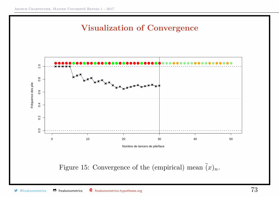
Figure 15: Convergence of the (empirical) mean (x)n.
@freakonometrics freakonometrics freakonometrics.hypotheses.org 73
Arthur Charpentier, Master Université Rennes 1 - 2017
Visualization of Convergence
0 10 20 30 40 50
0.0
0.2
0.4
0.6
0.8
1.0
Nombre de lancers de pile/face
Fré
quen
ce d
es p
ile
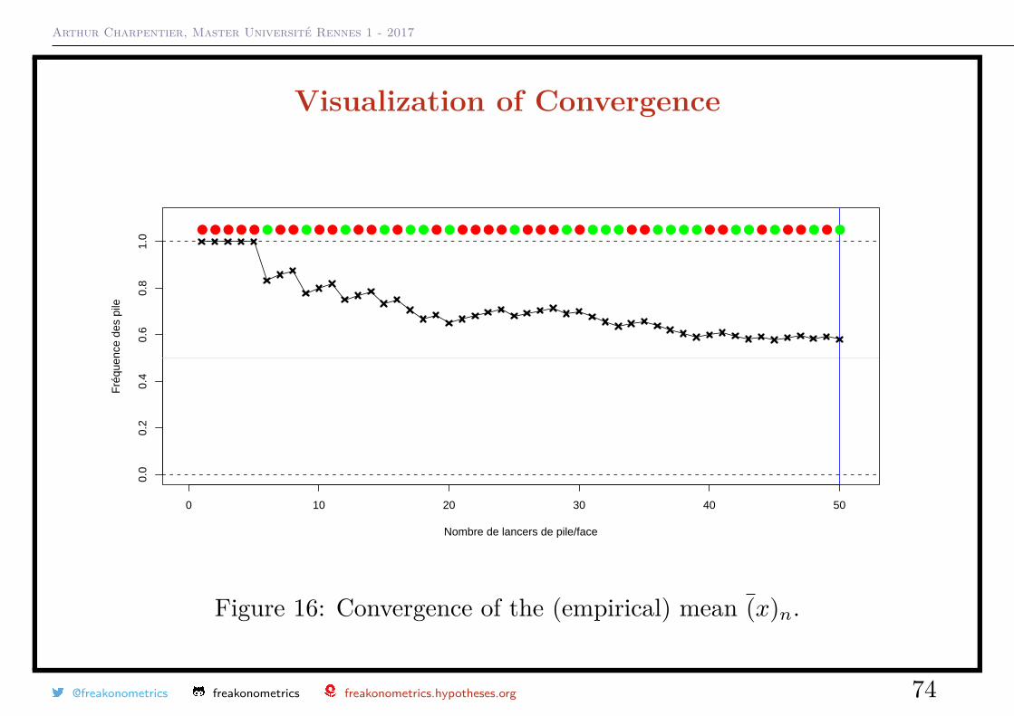
Figure 16: Convergence of the (empirical) mean (x)n.
@freakonometrics freakonometrics freakonometrics.hypotheses.org 74
Arthur Charpentier, Master Université Rennes 1 - 2017
Visualization of Convergence
0 10 20 30 40 50
0.0
0.2
0.4
0.6
0.8
1.0
Nombre de lancers de pile/face
Fré
quen
ce d
es p
ile
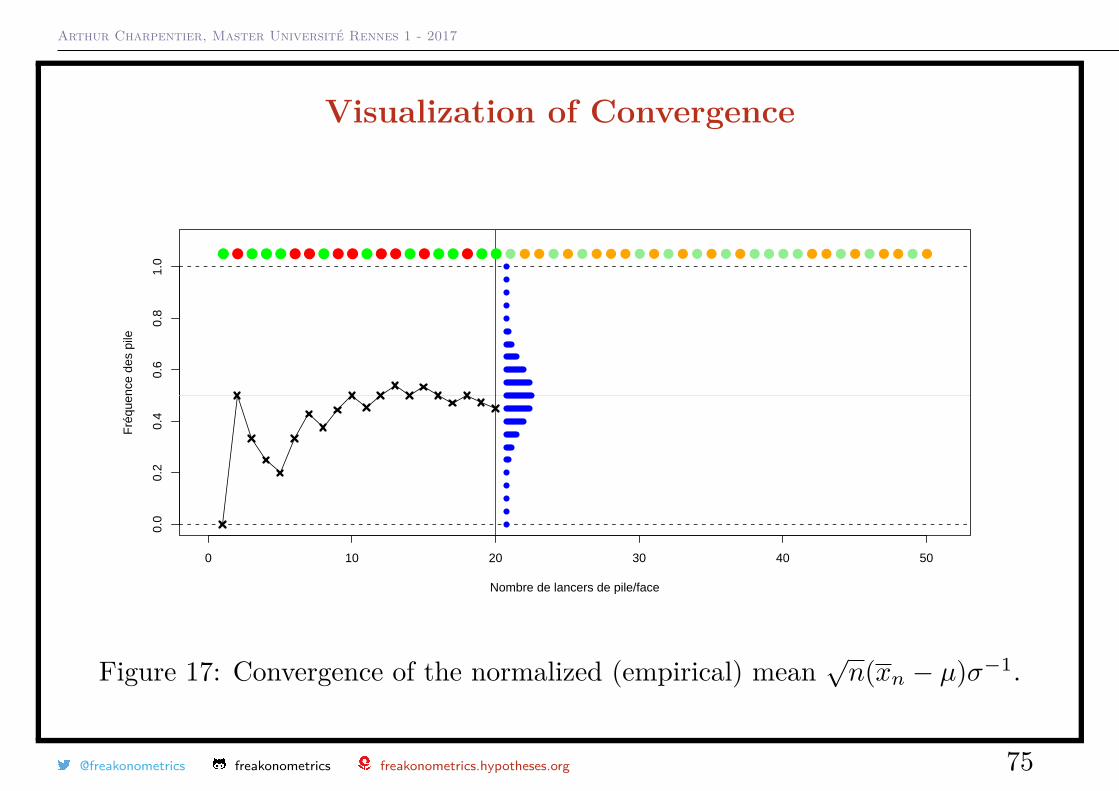
Figure 17: Convergence of the normalized (empirical) mean√n(xn − µ)σ−1.
@freakonometrics freakonometrics freakonometrics.hypotheses.org 75
Arthur Charpentier, Master Université Rennes 1 - 2017
Visualization of Convergence
0 10 20 30 40 50
0.0
0.2
0.4
0.6
0.8
1.0
Nombre de lancers de pile/face
Fré
quen
ce d
es p
ile
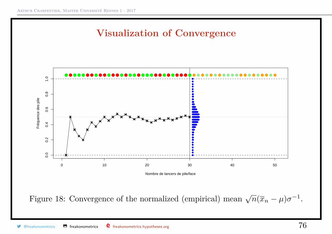
Figure 18: Convergence of the normalized (empirical) mean√n(xn − µ)σ−1.
@freakonometrics freakonometrics freakonometrics.hypotheses.org 76
Arthur Charpentier, Master Université Rennes 1 - 2017
Visualization of Convergence
0 10 20 30 40 50
0.0
0.2
0.4
0.6
0.8
1.0
Nombre de lancers de pile/face
Fré
quen
ce d
es p
ile
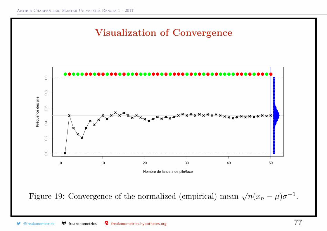
Figure 19: Convergence of the normalized (empirical) mean√n(xn − µ)σ−1.
@freakonometrics freakonometrics freakonometrics.hypotheses.org 77
Arthur Charpentier, Master Université Rennes 1 - 2017
From Convergence to ApproximationsProposition. Let (Xn) denote a sequence of i.i.d. random variables B(n, p). Ifn→∞ and p→ 0 with p ∼ λ/n, Xn
L→ X where X ∼ P(λ).
Proof. Based on (n
k
)pk[1− p]n−k ≈ exp[−np] [np]
k
k!
Poisson distribution P(np) is a good approximation of the Binomial B(n, p) whenn is large, as well as np→∞ (and thus p small, with respect to n).
In practice, it can be used when n > 30 and np < 5.
@freakonometrics freakonometrics freakonometrics.hypotheses.org 78
Arthur Charpentier, Master Université Rennes 1 - 2017
From convergence to approximationsProposition. Let (Xn) be a sequence of i.i.d. B(n, p) varialbes. Then ifnp→∞, [Xn − np]/
√np(1− p) L→ X with X ∼ N (0, 1).
In practice, the approximation is valid for n > 30 and np > 5, and n(1− p) > 5.
The Gaussian distribution N (np, np(1− p)) is an approximation of the Binomialdistribution B(n, p) for n large enough, with np, n(1− p)→∞.
@freakonometrics freakonometrics freakonometrics.hypotheses.org 79
Arthur Charpentier, Master Université Rennes 1 - 2017
From convergence to approximations
0 2 4 6 8 10
0.00
0.10
0.20
P((X
==x))
0 5 10 15 20
0.00
0.04
0.08
0.12
10 20 30 40
0.00
0.04
0.08
x
P((X
==x))
20 30 40 50 60
0.00
0.02
0.04
0.06
x
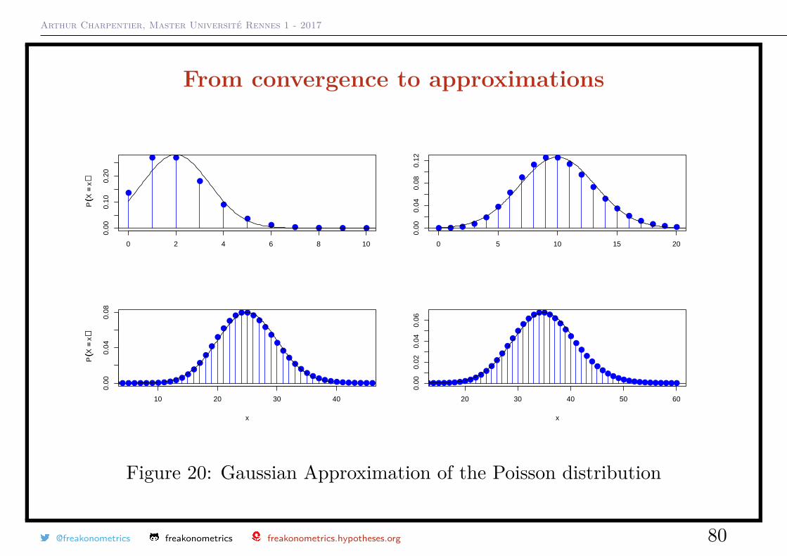
Figure 20: Gaussian Approximation of the Poisson distribution
@freakonometrics freakonometrics freakonometrics.hypotheses.org 80
Arthur Charpentier, Master Université Rennes 1 - 2017
Transforming Random VariablesLet X be an absolutely continuous random variable with density f(x). We wantto know the distribution ofY = φ(X).Proposition. If function φ is a differentiable one-to-one mapping, then variableY has a density g satisfying
g(y) = f(φ−1(y))φ′(φ−1(y)) .
Transforming Random VariablesProposition. Let X be an absolutely continuous random variable with cdf F ,i.e. F (x) = P(X ≤ x). Then Y = F (X) has a uniform distribution on [0, 1].Proposition. Let Y be a uniform distribution on [0, 1] and F denote a cdf.Then X = F−1(Y ) is a random variable with cdf F .
This will be the startig point of Monte Carlo simulations.
@freakonometrics freakonometrics freakonometrics.hypotheses.org 81
Arthur Charpentier, Master Université Rennes 1 - 2017
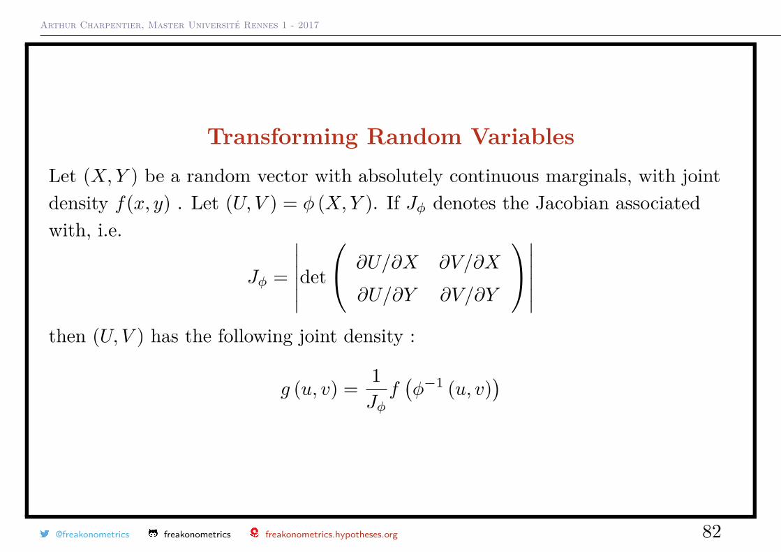
Transforming Random VariablesLet (X,Y ) be a random vector with absolutely continuous marginals, with jointdensity f(x, y) . Let (U, V ) = φ (X,Y ). If Jφ denotes the Jacobian associatedwith, i.e.
Jφ =
∣∣∣∣∣∣det
∂U/∂X ∂V/∂X
∂U/∂Y ∂V/∂Y
∣∣∣∣∣∣then (U, V ) has the following joint density :
g (u, v) = 1Jφf(φ−1 (u, v)
)
@freakonometrics freakonometrics freakonometrics.hypotheses.org 82
Arthur Charpentier, Master Université Rennes 1 - 2017
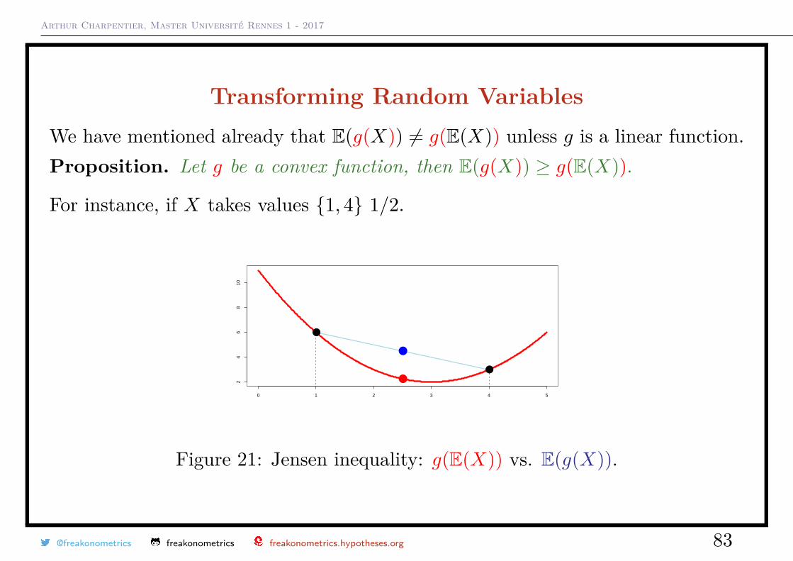
Transforming Random VariablesWe have mentioned already that E(g(X)) 6= g(E(X)) unless g is a linear function.Proposition. Let g be a convex function, then E(g(X)) ≥ g(E(X)).
For instance, if X takes values 1, 4 1/2.
0 1 2 3 4 5
24
68
10
Figure 21: Jensen inequality: g(E(X)) vs. E(g(X)).
@freakonometrics freakonometrics freakonometrics.hypotheses.org 83
Arthur Charpentier, Master Université Rennes 1 - 2017
Computer Based RandomnessCalculations of E[h(X)] can be complicated,
E[h(X)] =∫ ∞−∞
h(x)f(x)dx.
Sometimes, we simply want a numerical approximation of that integral. One canuse numerical functions to compute those integrals. But one can also use MonteCarlo techniques. Assume that we can generate a sample x1, · · · , xn, · · · i.i.d.from distribution F . From the law of large numbers we know that
1n
n∑i=1
h(x)→ E[h(X)], as n→∞.
or1n
n∑i=1
h(F−1X (ui))→ E[h(X)], as n→∞
if x1, · · · , xn, · · · i.i.d. from a uniform distribution on [0, 1].
@freakonometrics freakonometrics freakonometrics.hypotheses.org 84
Arthur Charpentier, Master Université Rennes 1 - 2017
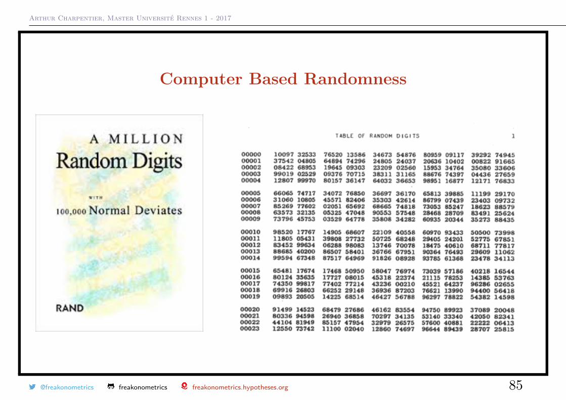
Computer Based Randomness
@freakonometrics freakonometrics freakonometrics.hypotheses.org 85
Arthur Charpentier, Master Université Rennes 1 - 2017
Monte Carlo SimulationsLet X ∼ Cauchy what is P[X > 2]? Let
p = P[X > 2] =∫ ∞
2
dx
π(1 + x2) (∼ 0.15)
since f(x) = 1π(1 + x2) and Q(u) = F−1(u) = tan
(π[u− 1
2]).
Crude Monte Carlo: use the law of large numbers
p1 = 1n
n∑i=1
1(Q(ui) > 2)
where ui are obtained from i.id. U([0, 1]) variables.
Observe that Var[p1] ∼ 0.127n .
Crude Monte Carlo (with symmetry): P[X > 2] = P[|X| > 2]/2 and use the law
@freakonometrics freakonometrics freakonometrics.hypotheses.org 86
Arthur Charpentier, Master Université Rennes 1 - 2017
of large numbers
p2 = 12n
n∑i=1
1(|Q(ui)| > 2)
where ui are obtained from i.id. U([0, 1]) variables.
Observe that Var[p2] ∼ 0.052n .
Using integral symmetries :∫ ∞2
dx
π(1 + x2) = 12 −
∫ 2
0
dx
π(1 + x2)
where the later integral is E[h(2U)] where h(x) = 2π(1 + x2) .
From the law of large numbers
p3 = 12 −
1n
n∑i=1
h(2ui)
where ui are obtained from i.id. U([0, 1]) variables.
@freakonometrics freakonometrics freakonometrics.hypotheses.org 87
Arthur Charpentier, Master Université Rennes 1 - 2017
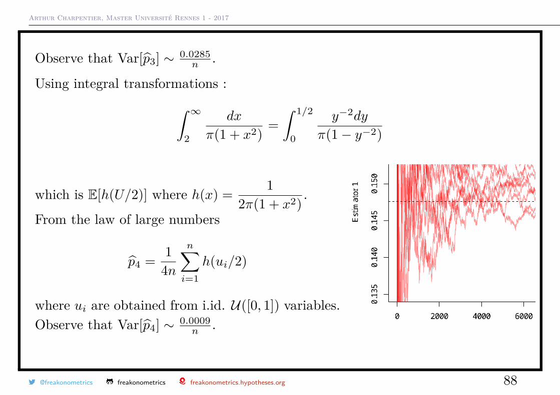
Observe that Var[p3] ∼ 0.0285n .
Using integral transformations :∫ ∞2
dx
π(1 + x2) =∫ 1/2
0
y−2dy
π(1− y−2)
which is E[h(U/2)] where h(x) = 12π(1 + x2) .
From the law of large numbers
p4 = 14n
n∑i=1
h(ui/2)
where ui are obtained from i.id. U([0, 1]) variables.Observe that Var[p4] ∼ 0.0009
n .
@freakonometrics freakonometrics freakonometrics.hypotheses.org 88
Arthur Charpentier, Master Université Rennes 1 - 2017
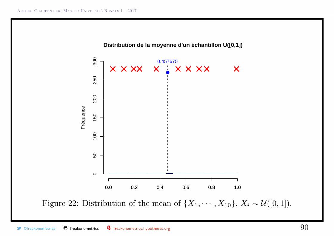
The Estimator as a Random VariableIn descriptive statistics, estimators are functions of the observed sample,x1, · · · , xn, e.g.
xn = x1 + · · ·+ xnn
In mathematical statistics, assume that xi = Xi(ω), i.e. realizations of randomvariables,
Xn = X1 + · · ·+Xn
n
X1,..., Xn being random variables, so that Xn is also a random variable.
For example, assume that we have a sample of size n = 20 from a uniformdistribution on [0, 1].
@freakonometrics freakonometrics freakonometrics.hypotheses.org 89
Arthur Charpentier, Master Université Rennes 1 - 2017
Distribution de la moyenne d'un échantillon U([0,1])
Fré
quen
ce
0.0 0.2 0.4 0.6 0.8 1.0
050
100
150
200
250
300
0.457675
0.0 0.2 0.4 0.6 0.8 1.0
Figure 22: Distribution of the mean of X1, · · · , X10, Xi ∼ U([0, 1]).
@freakonometrics freakonometrics freakonometrics.hypotheses.org 90
Arthur Charpentier, Master Université Rennes 1 - 2017
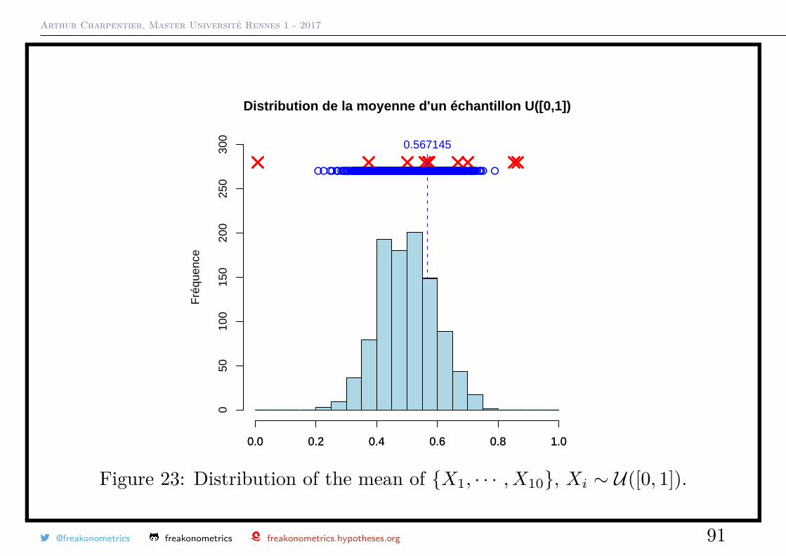
Distribution de la moyenne d'un échantillon U([0,1])
Fré
quen
ce
0.0 0.2 0.4 0.6 0.8 1.0
050
100
150
200
250
300
0.567145
0.0 0.2 0.4 0.6 0.8 1.0
Figure 23: Distribution of the mean of X1, · · · , X10, Xi ∼ U([0, 1]).
@freakonometrics freakonometrics freakonometrics.hypotheses.org 91
Arthur Charpentier, Master Université Rennes 1 - 2017
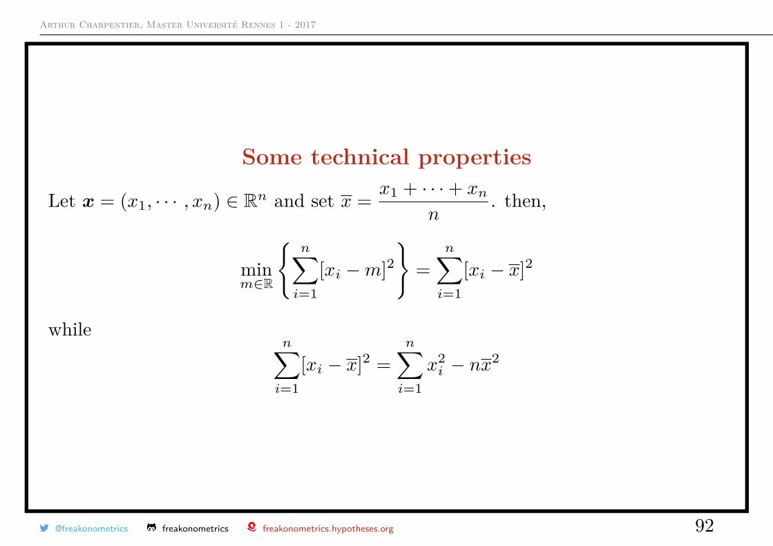
Some technical properties
Let x = (x1, · · · , xn) ∈ Rn and set x = x1 + · · ·+ xnn
. then,
minm∈R
n∑i=1
[xi −m]2
=n∑i=1
[xi − x]2
whilen∑i=1
[xi − x]2 =n∑i=1
x2i − nx2
@freakonometrics freakonometrics freakonometrics.hypotheses.org 92
Arthur Charpentier, Master Université Rennes 1 - 2017
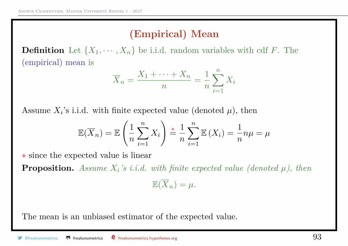
(Empirical) MeanDefinition Let X1, · · · , Xn be i.i.d. random variables with cdf F . The(empirical) mean is
Xn = X1 + · · ·+Xn
n= 1n
n∑i=1
Xi
Assume Xi’s i.i.d. with finite expected value (denoted µ), then
E(Xn) = E
(1n
n∑i=1
Xi
)∗= 1n
n∑i=1
E (Xi) = 1nnµ = µ
∗ since the expected value is linearProposition. Assume Xi’s i.i.d. with finite expected value (denoted µ), then
E(Xn) = µ.
The mean is an unbiased estimator of the expected value.
@freakonometrics freakonometrics freakonometrics.hypotheses.org 93
Arthur Charpentier, Master Université Rennes 1 - 2017
(Empirical) VarianceAssume Xi’s i.i.d. with finite variance (denoted σ2), then
Var(Xn) = Var(
1n
n∑i=1
Xi
)∗= 1n2
n∑i=1
Var (Xi) = 1n2nσ
2 = σ2
n
∗ because variables are independent, and variance is a quadratic function.Proposition. Assume Xi’s i.i.d. with finite variance (denoted σ2),
Var(Xn) = σ2
n.
@freakonometrics freakonometrics freakonometrics.hypotheses.org 94
Arthur Charpentier, Master Université Rennes 1 - 2017
(Empirical) VarianceDefinition Let X1, · · · , Xn be n i.i.d. random variables with distribution F .The empirical variance is
S2n = 1
n− 1
n∑i=1
[Xi −Xn]2.
Assume Xi’s i.i.d. with finite variance (denoted σ2),
E(S2n) = E
(1
n− 1
n∑i=1
[Xi −Xn]2)∗= E
(1
n− 1
[n∑i=1
X2i − nX
2n
])∗ from the same property as before
E(S2n) = 1
n− 1 [nE(X2i )− nE(X2)] ∗= 1
n− 1
[n(σ2 + µ2)− n
(σ2
n+ µ2
)]= σ2
∗ since Var(X) = E(X2)− E(X)2
@freakonometrics freakonometrics freakonometrics.hypotheses.org 95
Arthur Charpentier, Master Université Rennes 1 - 2017
(Empirical) VarianceProposition. Asusme that Xi independent, with finite variance (denoted σ2),
E(S2n) = σ2.
Empirical variance is an unbiased estimator of the variance.
Note that
S2n = 1
n
n∑i=1
[Xi −Xn]2
is also a popular estimator (but biased).
@freakonometrics freakonometrics freakonometrics.hypotheses.org 96
Arthur Charpentier, Master Université Rennes 1 - 2017
Gaussian SamplingProposition. Suppose Xi’s i.i.d. from a N (µ, σ2) distribution, then
• Xn and S2n are independent random variables
• Xn has distribution N(µ,σ2
n
)• (n− 1)S2
n/σ2 has distribution χ2(n− 1). Assume that Xi’s are i.i.d. random
variables with distribution N (µ, σ2), then
•√nXn − µ
σhas a N (0, 1) distribution
•√nXn − µSn
has a Student-t distribution with n− 1 degrees of freedom
@freakonometrics freakonometrics freakonometrics.hypotheses.org 97
Arthur Charpentier, Master Université Rennes 1 - 2017
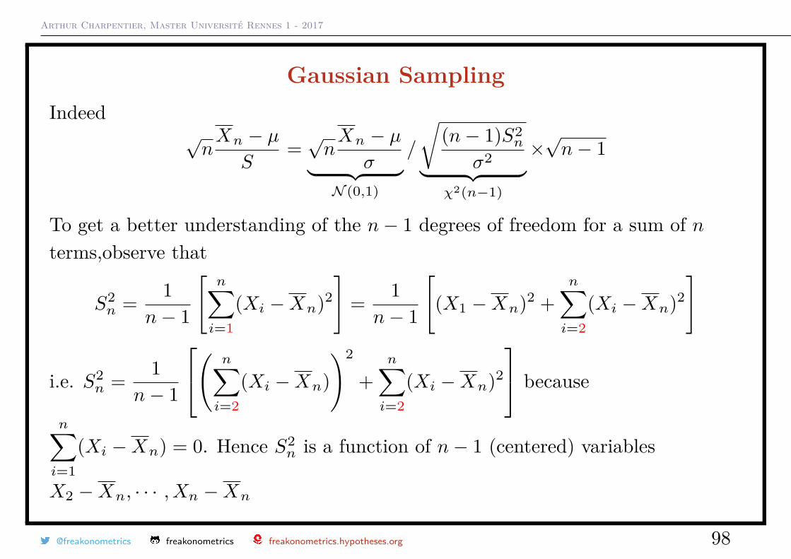
Gaussian SamplingIndeed
√nXn − µS
=√nXn − µ
σ︸ ︷︷ ︸N (0,1)
/
√(n− 1)S2
n
σ2︸ ︷︷ ︸χ2(n−1)
×√n− 1
To get a better understanding of the n− 1 degrees of freedom for a sum of nterms,observe that
S2n = 1
n− 1
[n∑i=1
(Xi −Xn)2
]= 1n− 1
[(X1 −Xn)2 +
n∑i=2
(Xi −Xn)2
]
i.e. S2n = 1
n− 1
( n∑i=2
(Xi −Xn))2
+n∑i=2
(Xi −Xn)2
because
n∑i=1
(Xi −Xn) = 0. Hence S2n is a function of n− 1 (centered) variables
X2 −Xn, · · · , Xn −Xn
@freakonometrics freakonometrics freakonometrics.hypotheses.org 98
Arthur Charpentier, Master Université Rennes 1 - 2017
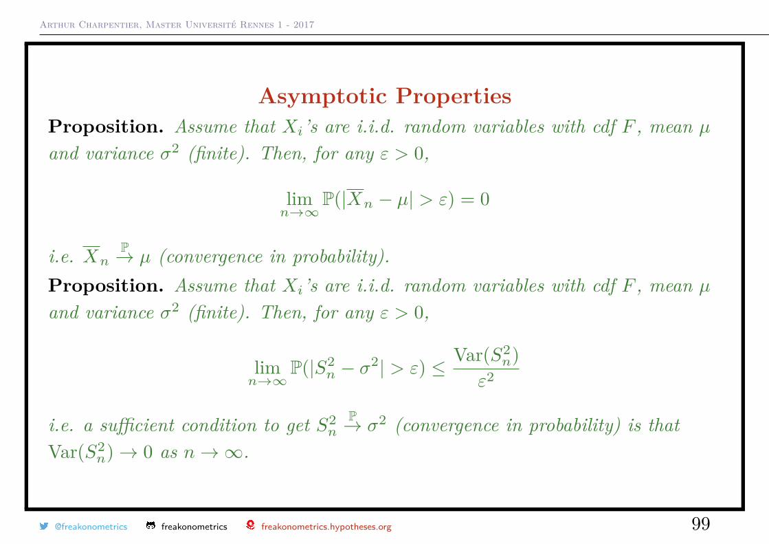
Asymptotic PropertiesProposition. Assume that Xi’s are i.i.d. random variables with cdf F , mean µand variance σ2 (finite). Then, for any ε > 0,
limn→∞
P(|Xn − µ| > ε) = 0
i.e. XnP→ µ (convergence in probability).
Proposition. Assume that Xi’s are i.i.d. random variables with cdf F , mean µand variance σ2 (finite). Then, for any ε > 0,
limn→∞
P(|S2n − σ2| > ε) ≤ Var(S2
n)ε2
i.e. a sufficient condition to get S2n
P→ σ2 (convergence in probability) is thatVar(S2
n)→ 0 as n→∞.
@freakonometrics freakonometrics freakonometrics.hypotheses.org 99

Arthur Charpentier, Master Université Rennes 1 - 2017
Asymptotic PropertiesProposition. Assume that Xi’s are i.i.d. random variables with cdf F , mean µand variance σ2 (finite). Then for any z ∈ R,
limn→∞
P(√
nXn − µ
σ≤ z)
=∫ z
−∞
1√2π
exp(− t
2
2
)dt
i.e.√nXn − µ
σ
L→ N (0, 1).
Remark If Xi’s have a N (µ, σ2) distribution, then
√nXn − µ
σ∼ N (0, 1).
@freakonometrics freakonometrics freakonometrics.hypotheses.org 100
Arthur Charpentier, Master Université Rennes 1 - 2017
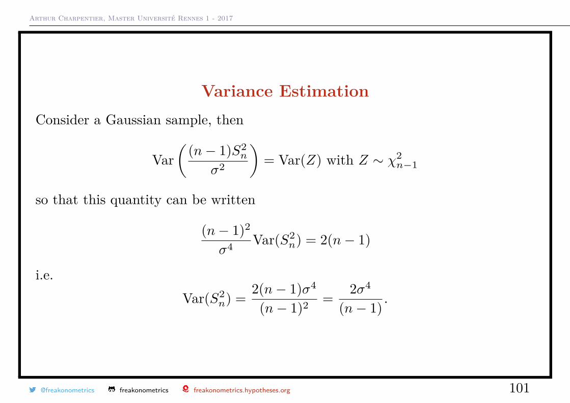
Variance EstimationConsider a Gaussian sample, then
Var(
(n− 1)S2n
σ2
)= Var(Z) with Z ∼ χ2
n−1
so that this quantity can be written
(n− 1)2
σ4 Var(S2n) = 2(n− 1)
i.e.Var(S2
n) = 2(n− 1)σ4
(n− 1)2 = 2σ4
(n− 1) .
@freakonometrics freakonometrics freakonometrics.hypotheses.org 101
Arthur Charpentier, Master Université Rennes 1 - 2017
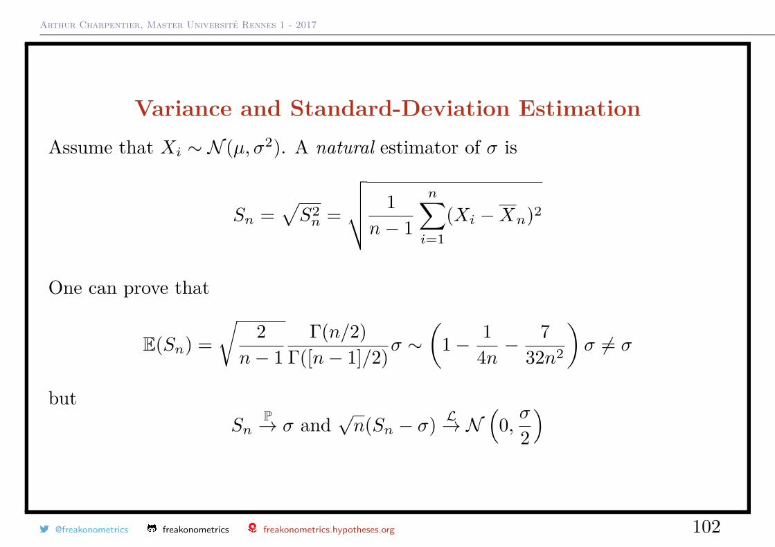
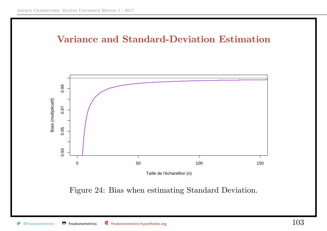
Variance and Standard-Deviation EstimationAssume that Xi ∼ N (µ, σ2). A natural estimator of σ is
Sn =√S2n =
√√√√ 1n− 1
n∑i=1
(Xi −Xn)2
One can prove that
E(Sn) =√
2n− 1
Γ(n/2)Γ([n− 1]/2)σ ∼
(1− 1
4n −7
32n2
)σ 6= σ
butSn
P→ σ and√n(Sn − σ) L→ N
(0, σ2
)
@freakonometrics freakonometrics freakonometrics.hypotheses.org 102
Arthur Charpentier, Master Université Rennes 1 - 2017
Variance and Standard-Deviation Estimation
0 50 100 150
0.93
0.95
0.97
0.99
Taille de l'échantillon (n)
Bia
is (
mul
tiplic
atif)
Figure 24: Bias when estimating Standard Deviation.
@freakonometrics freakonometrics freakonometrics.hypotheses.org 103
Arthur Charpentier, Master Université Rennes 1 - 2017
Transformed SampleLet g : R→ R be sufficiently regular to write Taylor expansion
g(x) = g(x0) + g′(x0) · [x− x0] + some (small) additional term
Let Yi = g(Xi). The, if E(Xi) = µ with g′(µ) 6= 0
Yi = g(Xi) ≈ g(µ) + g′(µ) · [Xi − µ]
so thatE(Yi) = E(g(Xi)) ≈ g(µ)
andVar(Yi) = Var(g(Xi)) ≈ [g′(µ)]2Var(Xi)
Keep in mind that those are just approximations.
@freakonometrics freakonometrics freakonometrics.hypotheses.org 104
Arthur Charpentier, Master Université Rennes 1 - 2017
Transformed SampleThe Delta-Method can be used to derived asymptotic propertiesProposition. Suppose Xi’s i.i.d. with distribution F , expected value µ andvariance σ2 (finite), then
√n(Xn − µ) L→ N (0, σ2)
And if g′(µ) 6= 0, then√n(g(Xn)− g(µ)) L→ N (0, [g′(µ)]2σ2)
Proposition. Suppose Xi’s i.i.d. with distribution F , expected value µ andvariance σ2 (finite), then if g′(µ) = 0 but g′′(µ) 6= 0, we have
√n(g(Xn)− g(µ)) L→ g′′(µ)
2 σ2χ2(1)
@freakonometrics freakonometrics freakonometrics.hypotheses.org 105
Arthur Charpentier, Master Université Rennes 1 - 2017
Transformed SampleFor example, if µ 6= 0,
E(
1Xn
)→ 1
µas n→∞
and√n
(1Xn
− 1µ
)L→ N
(0, 1µ4σ
2)
even ifE(
1Xn
)6= 1µ.
@freakonometrics freakonometrics freakonometrics.hypotheses.org 106
Arthur Charpentier, Master Université Rennes 1 - 2017
Confidence Interval for µThe l’intervalle de confiance for µ of order 1− α (e.g. 95%) is the smallestinterval I such that
P(µ ∈ I) = 1− α.
Let uα denote the quantile of the N (0, 1) of order α, i.e.
uα/2 = −u1−α/2 = Φ−1(α/2).
since Z =√nXn − µ
σ∼ N (0, 1), we get P(Z ∈ [uα/2, u1−α/2]) = 1− α, and
P(µ ∈
[X +
uα/2√nσ,X +
u1−α/2√n
σ
])= 1− α.
@freakonometrics freakonometrics freakonometrics.hypotheses.org 107
Arthur Charpentier, Master Université Rennes 1 - 2017
Confidence Interval, mean of a Gaussian Sample
• if α = 10%, u1−α/2 = 1.64 and therefore, with probability 90%,
X − 1.64√nσ ≤ µ ≤ X + 1.64√
nσ,
• if α = 5%, u1−α/2 = 1.96 and therefore, with probability 95%,
X − 1.96√nσ ≤ µ ≤ X + 1.96√
nσ,
@freakonometrics freakonometrics freakonometrics.hypotheses.org 108
Arthur Charpentier, Master Université Rennes 1 - 2017
Confidence Interval, mean of a Gaussian Sample
If variance is unknown, plug-in S2n = 1
n− 1
(n∑i=1
X2i
)−X2
n.
We’ve seen that
(n− 1)S2n
σ2 =n∑i=1
Xi − E(X)σ︸ ︷︷ ︸
N (0,1)
2
︸ ︷︷ ︸χ2(n) distribution
−
Xn − E(X)σ/√n︸ ︷︷ ︸
N (0,1)
2
︸ ︷︷ ︸χ2(1) distribution
From Cochrane theorem (n− 1)S2n
σ2 ∼ χ2(n− 1).
@freakonometrics freakonometrics freakonometrics.hypotheses.org 109
Arthur Charpentier, Master Université Rennes 1 - 2017
Confidence Interval, mean of a Gaussian SampleSince Xn and S2
n are independent,
T =√n− 1Xn − µ
Sn=
Xn−µσ/√n−1√
(n−1)S2n
(n−1)σ2
∼ St(n− 1).
If t(n−1)α/2 denote the quantile of the St(n− 1) distribution with level α/2, i.e.
t(n)α/2 = −t(n−1)
1−α/2 satisfies P(T ≤ t(n−1)α/2 ) = α/2
thus P(T ∈ [t(n−1)α/2 , t
(n−1)1−α/2]) = 1− α, and therefore
P
µ ∈X +
t(n−1)α/2√n− 1
σ,X +t(n−1)1−α/2√n− 1
σ
= 1− α.
@freakonometrics freakonometrics freakonometrics.hypotheses.org 110
Arthur Charpentier, Master Université Rennes 1 - 2017
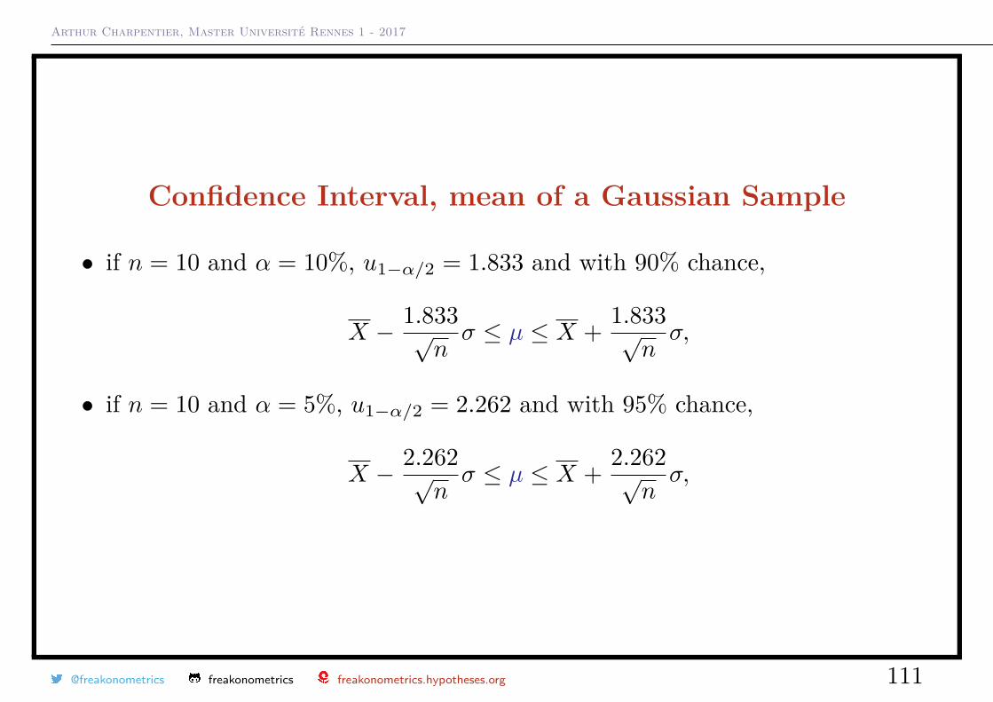
Confidence Interval, mean of a Gaussian Sample
• if n = 10 and α = 10%, u1−α/2 = 1.833 and with 90% chance,
X − 1.833√nσ ≤ µ ≤ X + 1.833√
nσ,
• if n = 10 and α = 5%, u1−α/2 = 2.262 and with 95% chance,
X − 2.262√nσ ≤ µ ≤ X + 2.262√
nσ,
@freakonometrics freakonometrics freakonometrics.hypotheses.org 111
Arthur Charpentier, Master Université Rennes 1 - 2017
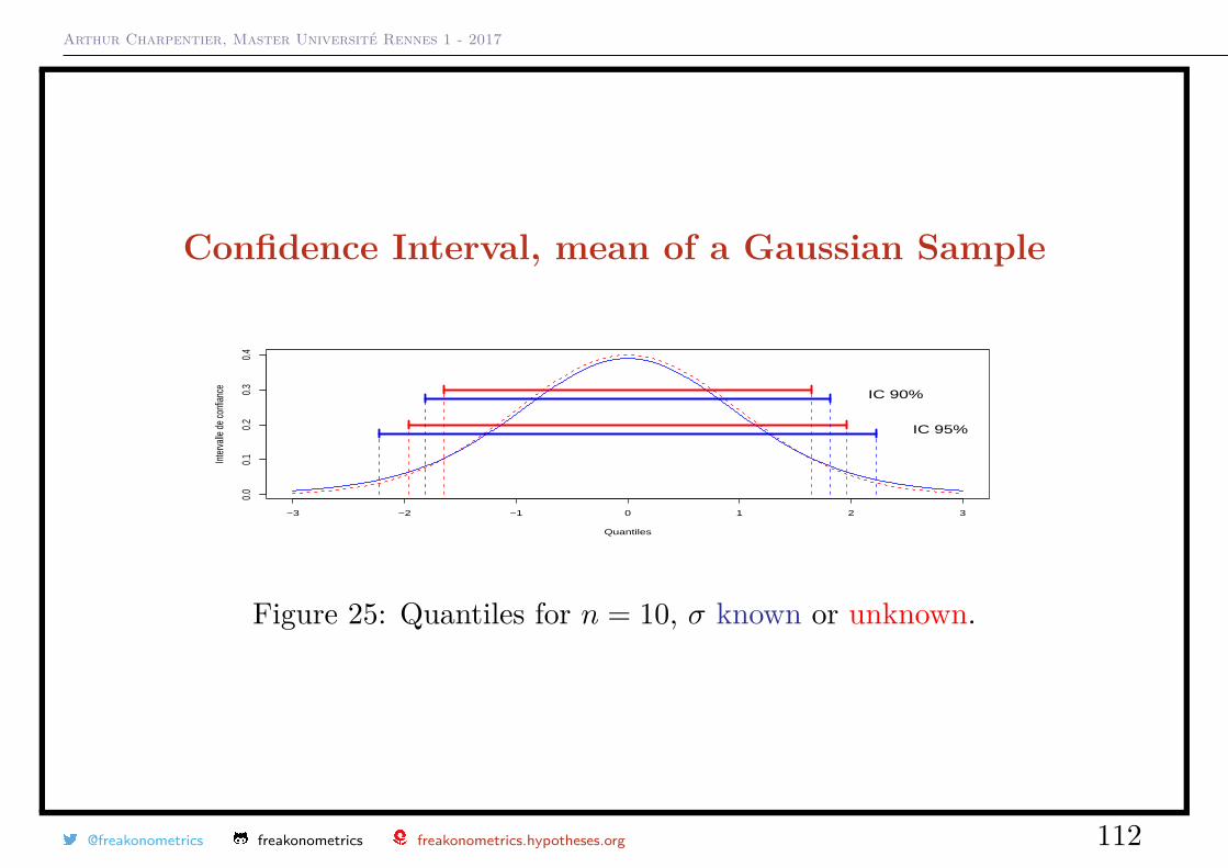
Confidence Interval, mean of a Gaussian Sample
−3 −2 −1 0 1 2 3
0.0
0.1
0.2
0.3
0.4
Quantiles
Inte
rvall
e de
conf
iance IC 90%
IC 95%
Figure 25: Quantiles for n = 10, σ known or unknown.
@freakonometrics freakonometrics freakonometrics.hypotheses.org 112

Arthur Charpentier, Master Université Rennes 1 - 2017
Confidence Interval, mean of a Gaussian Sample
• if n = 20 and α = 10%, u1−α/2 = 1.729 and thus, with 90% chance
X − 1.729√nσ ≤ µ ≤ X + 1.729√
nσ,
• if n = 20 and α = 10%, u1−α/2 = 1.729 and thus, with 95% chance
X − 2.093√nσ ≤ µ ≤ X + 2.093√
nσ,
@freakonometrics freakonometrics freakonometrics.hypotheses.org 113

Arthur Charpentier, Master Université Rennes 1 - 2017
Confidence Interval, mean of a Gaussian Sample
−3 −2 −1 0 1 2 3
0.0
0.1
0.2
0.3
0.4
Quantiles
Inte
rvall
e de
conf
iance IC 90%
IC 95%
Figure 26: Quantiles for n = 20, σ known or unknown.
@freakonometrics freakonometrics freakonometrics.hypotheses.org 114
Arthur Charpentier, Master Université Rennes 1 - 2017
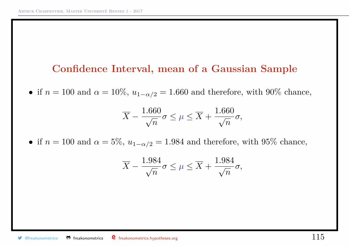
Confidence Interval, mean of a Gaussian Sample
• if n = 100 and α = 10%, u1−α/2 = 1.660 and therefore, with 90% chance,
X − 1.660√nσ ≤ µ ≤ X + 1.660√
nσ,
• if n = 100 and α = 5%, u1−α/2 = 1.984 and therefore, with 95% chance,
X − 1.984√nσ ≤ µ ≤ X + 1.984√
nσ,
@freakonometrics freakonometrics freakonometrics.hypotheses.org 115

Arthur Charpentier, Master Université Rennes 1 - 2017
Confidence Interval, mean of a Gaussian Sample
−3 −2 −1 0 1 2 3
0.0
0.1
0.2
0.3
0.4
Quantiles
Inte
rvall
e de
conf
iance IC 90%
IC 95%
Figure 27: Quantiles for n = 100, σ known or unknown.
@freakonometrics freakonometrics freakonometrics.hypotheses.org 116
Arthur Charpentier, Master Université Rennes 1 - 2017
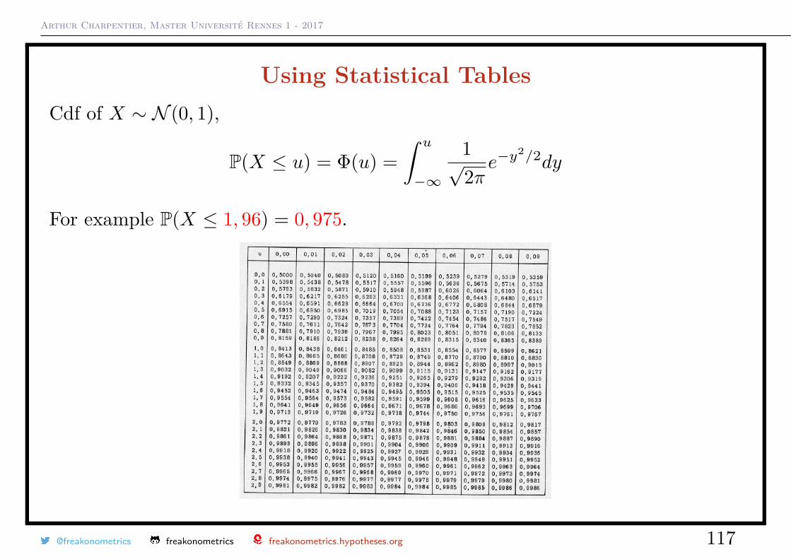
Using Statistical TablesCdf of X ∼ N (0, 1),
P(X ≤ u) = Φ(u) =∫ u
−∞
1√2πe−y
2/2dy
For example P(X ≤ 1, 96) = 0, 975.
@freakonometrics freakonometrics freakonometrics.hypotheses.org 117
Arthur Charpentier, Master Université Rennes 1 - 2017
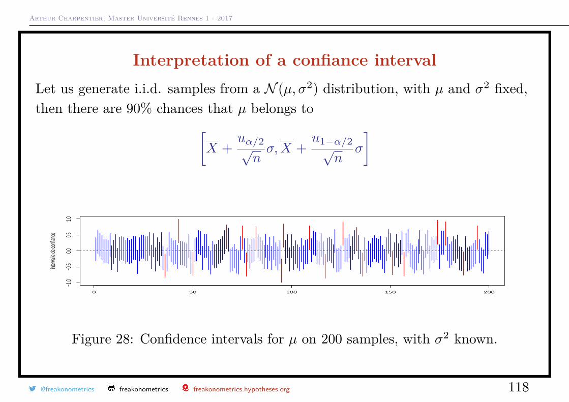
Interpretation of a confiance intervalLet us generate i.i.d. samples from a N (µ, σ2) distribution, with µ and σ2 fixed,then there are 90% chances that µ belongs to[
X +uα/2√nσ,X +
u1−α/2√n
σ
]
0 50 100 150 200
−1.0
−0.5
0.00.5
1.0
interv
alle de
confi
ance
Figure 28: Confidence intervals for µ on 200 samples, with σ2 known.
@freakonometrics freakonometrics freakonometrics.hypotheses.org 118
Arthur Charpentier, Master Université Rennes 1 - 2017
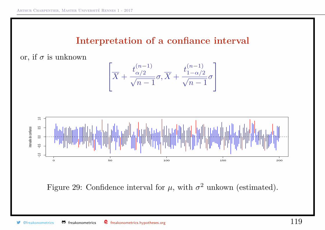
Interpretation of a confiance intervalor, if σ is unknown X +
t(n−1)α/2√n− 1
σ,X +t(n−1)1−α/2√n− 1
σ
0 50 100 150 200
−1.0
−0.5
0.00.5
1.0
interv
alle de
confi
ance
Figure 29: Confidence interval for µ, with σ2 unkown (estimated).
@freakonometrics freakonometrics freakonometrics.hypotheses.org 119
Arthur Charpentier, Master Université Rennes 1 - 2017
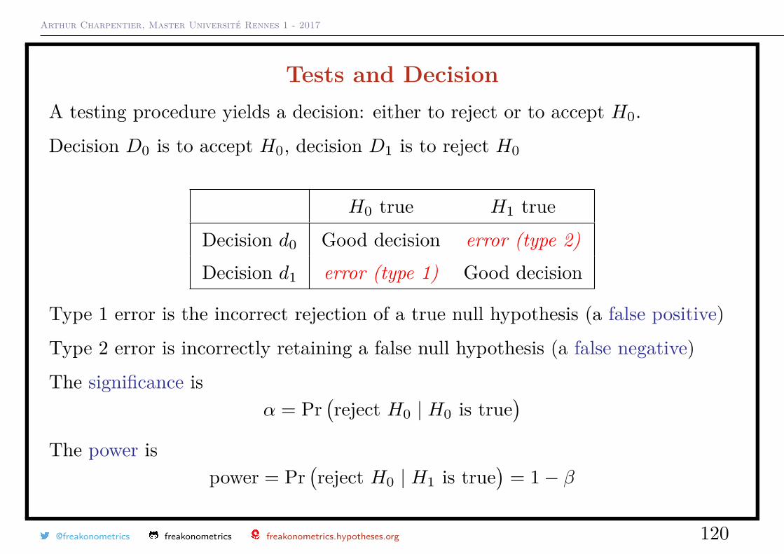
Tests and DecisionA testing procedure yields a decision: either to reject or to accept H0.
Decision D0 is to accept H0, decision D1 is to reject H0
H0 true H1 true
Decision d0 Good decision error (type 2)Decision d1 error (type 1) Good decision
Type 1 error is the incorrect rejection of a true null hypothesis (a false positive)
Type 2 error is incorrectly retaining a false null hypothesis (a false negative)
The significance isα = Pr
(reject H0 | H0 is true
)The power is
power = Pr(reject H0 | H1 is true
)= 1− β
@freakonometrics freakonometrics freakonometrics.hypotheses.org 120
Arthur Charpentier, Master Université Rennes 1 - 2017
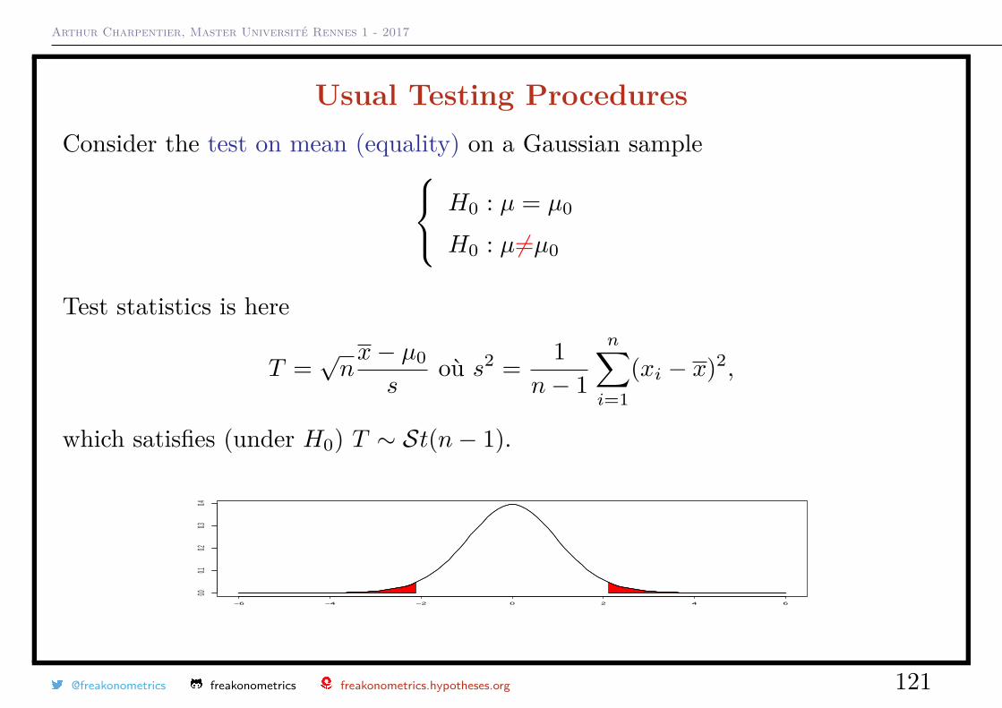
Usual Testing ProceduresConsider the test on mean (equality) on a Gaussian sample H0 : µ = µ0
H0 : µ6=µ0
Test statistics is here
T =√nx− µ0
soù s2 = 1
n− 1
n∑i=1
(xi − x)2,
which satisfies (under H0) T ∼ St(n− 1).
−6 −4 −2 0 2 4 6
0.00.1
0.20.3
0.4
@freakonometrics freakonometrics freakonometrics.hypotheses.org 121
Arthur Charpentier, Master Université Rennes 1 - 2017
Equal Means of Two (Independent) SamplesConsider a test of egality of means on two samples.
Consider two samples x1, · · · , xn and y1, · · · , ym. We wish to test H0 : µX = µY
H0 : µX 6=µY
Assume furthermore that Xi ∼ N (µX , σ2X) and Yj ∼ N (µY , σ2
Y ), i.e.
X ∼ N(µX ,
σ2X
n
)and Y ∼ N
(µY ,
σ2Y
m
)
@freakonometrics freakonometrics freakonometrics.hypotheses.org 122
Arthur Charpentier, Master Université Rennes 1 - 2017
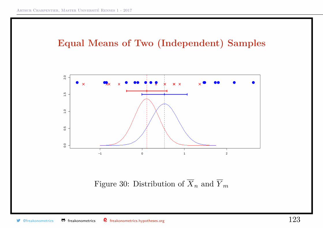
Equal Means of Two (Independent) Samples
−1 0 1 2
0.0
0.5
1.0
1.5
2.0
Figure 30: Distribution of Xn and Y m
@freakonometrics freakonometrics freakonometrics.hypotheses.org 123
Arthur Charpentier, Master Université Rennes 1 - 2017
Equal Means of Two (Independent) SamplesSince X and Y are independent, ∆ = X − Y has a Gaussian distribution,
E(∆) = µX − µY and Var(∆) = σ2X
n+ σ2
Y
m
Thus, under H0, µX − µY = 0 and thus
D ∼ N(
0, σ2X
n+ σ2
Y
m
),
i.e. ∆ = X − Y√σ2X
n+ σ2
Y
m
∼ N (0, 1).
@freakonometrics freakonometrics freakonometrics.hypotheses.org 124
Arthur Charpentier, Master Université Rennes 1 - 2017
Equal Means of Two (Independent) SamplesIf σ2
X and σ2Y are unknown: we will substitute estimators σ2
X et σ2Y ,
i.e. ∆ = X − Y√σ2X
n+ σ2
Y
m
∼ St(ν),
where ν is some complex (but known) function of n1 and n2.
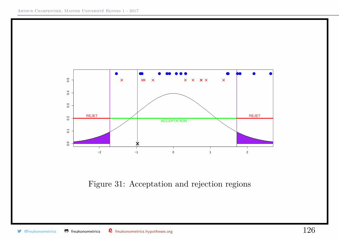
With acceptation rate α ∈ [0, 1] (e.g. 10%), accept H0 if tα/2 ≤ δ ≤ t1−α/2reject H0 if δ < tα/2 ou δ > t1−α/2
@freakonometrics freakonometrics freakonometrics.hypotheses.org 125
Arthur Charpentier, Master Université Rennes 1 - 2017
−2 −1 0 1 2
0.0
0.1
0.2
0.3
0.4
0.5
ACCEPTATIONREJET REJET
Figure 31: Acceptation and rejection regions
@freakonometrics freakonometrics freakonometrics.hypotheses.org 126
Arthur Charpentier, Master Université Rennes 1 - 2017
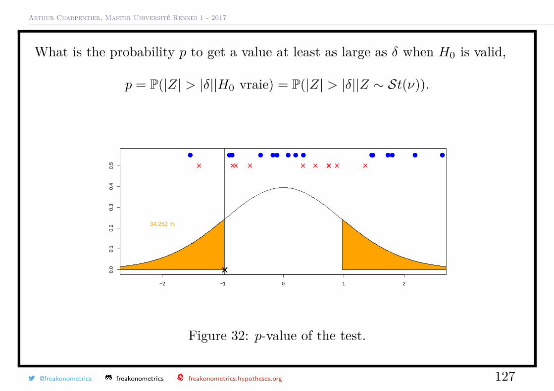
What is the probability p to get a value at least as large as δ when H0 is valid,
p = P(|Z| > |δ||H0 vraie) = P(|Z| > |δ||Z ∼ St(ν)).
−2 −1 0 1 2
0.0
0.1
0.2
0.3
0.4
0.5
34.252 %
Figure 32: p-value of the test.
@freakonometrics freakonometrics freakonometrics.hypotheses.org 127
Arthur Charpentier, Master Université Rennes 1 - 2017
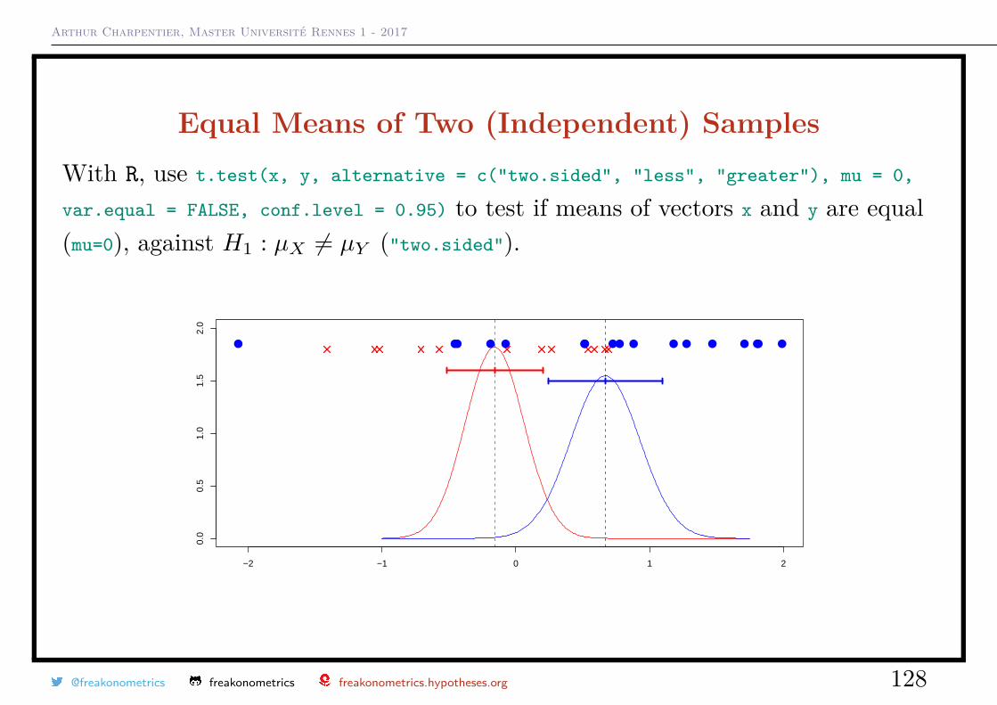
Equal Means of Two (Independent) SamplesWith R, use t.test(x, y, alternative = c("two.sided", "less", "greater"), mu = 0,
var.equal = FALSE, conf.level = 0.95) to test if means of vectors x and y are equal(mu=0), against H1 : µX 6= µY ("two.sided").
−2 −1 0 1 2
0.0
0.5
1.0
1.5
2.0
@freakonometrics freakonometrics freakonometrics.hypotheses.org 128
Arthur Charpentier, Master Université Rennes 1 - 2017
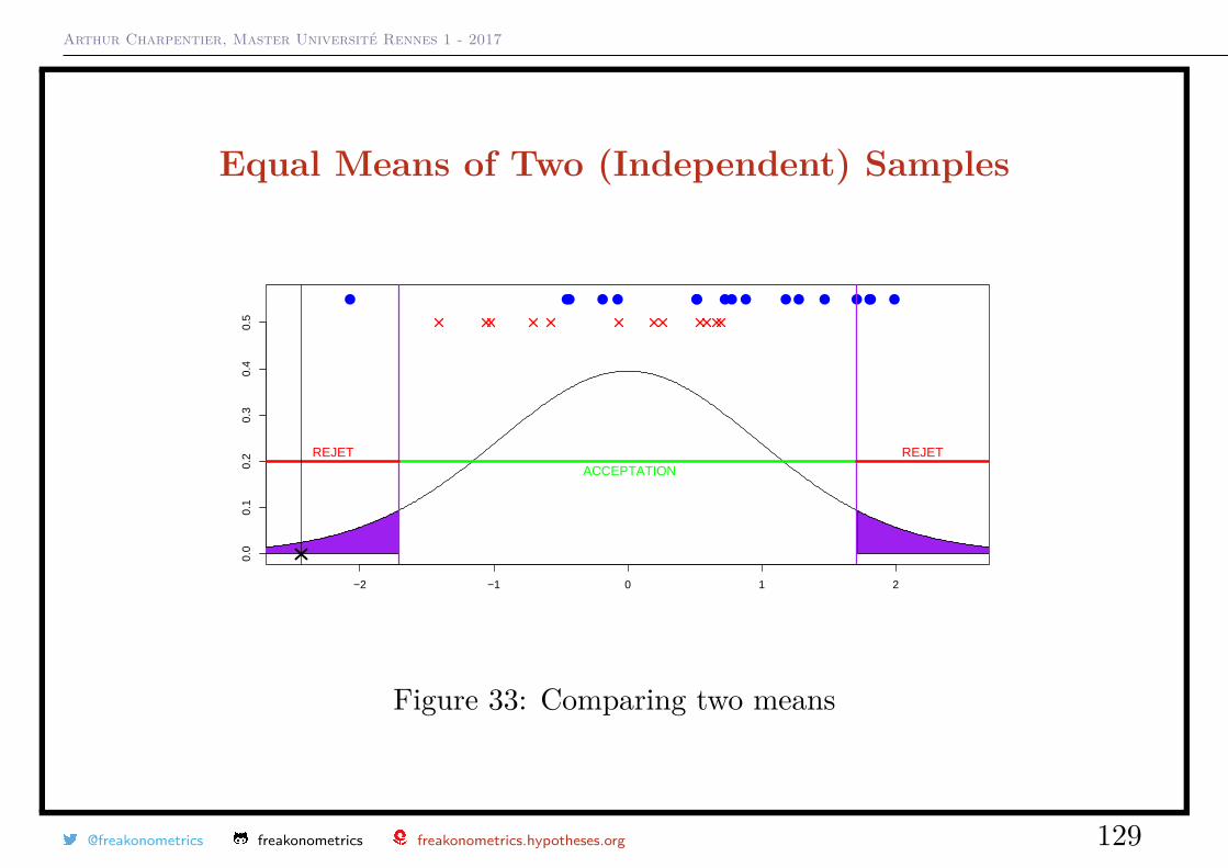
Equal Means of Two (Independent) Samples
−2 −1 0 1 2
0.0
0.1
0.2
0.3
0.4
0.5
ACCEPTATIONREJET REJET
Figure 33: Comparing two means
@freakonometrics freakonometrics freakonometrics.hypotheses.org 129
Arthur Charpentier, Master Université Rennes 1 - 2017
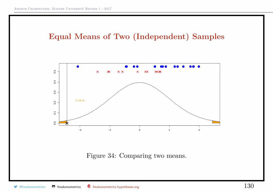
Equal Means of Two (Independent) Samples
−2 −1 0 1 2
0.0
0.1
0.2
0.3
0.4
0.5
2.19 %
Figure 34: Comparing two means.
@freakonometrics freakonometrics freakonometrics.hypotheses.org 130
Arthur Charpentier, Master Université Rennes 1 - 2017
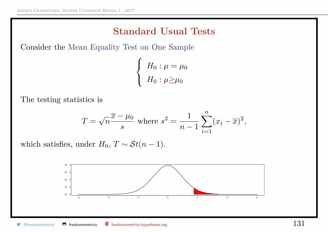
Standard Usual TestsConsider the Mean Equality Test on One Sample H0 : µ = µ0
H0 : µ≥µ0
The testing statistics is
T =√nx− µ0
swhere s2 = 1
n− 1
n∑i=1
(xi − x)2,
which satisfies, under H0, T ∼ St(n− 1).
−6 −4 −2 0 2 4 6
0.00.1
0.20.3
0.4
@freakonometrics freakonometrics freakonometrics.hypotheses.org 131
Arthur Charpentier, Master Université Rennes 1 - 2017
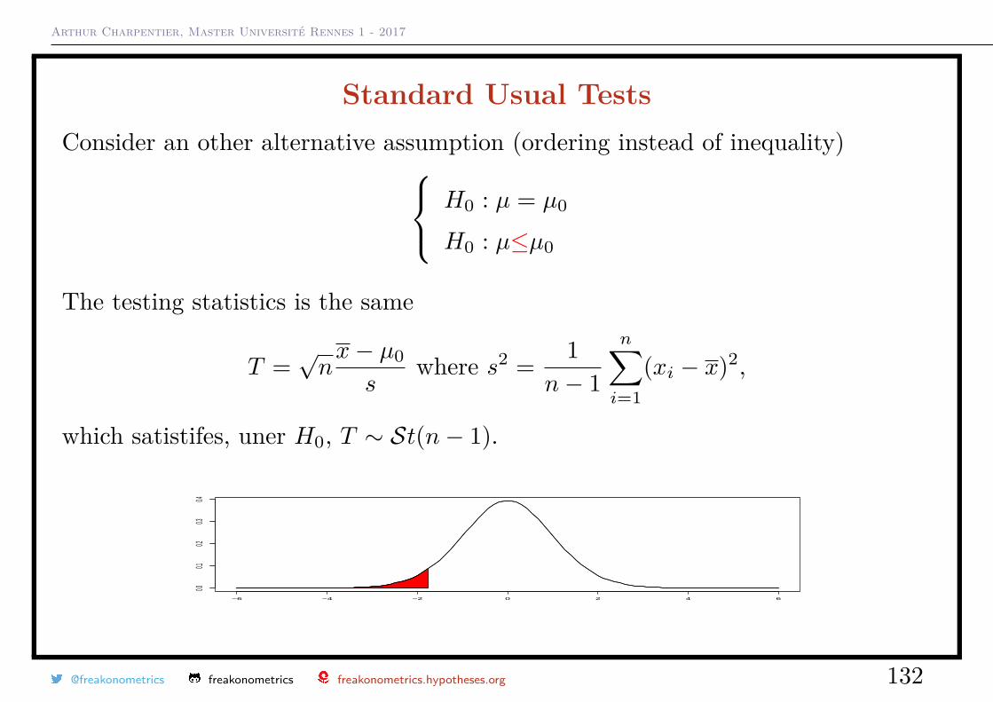
Standard Usual TestsConsider an other alternative assumption (ordering instead of inequality) H0 : µ = µ0
H0 : µ≤µ0
The testing statistics is the same
T =√nx− µ0
swhere s2 = 1
n− 1
n∑i=1
(xi − x)2,
which satistifes, uner H0, T ∼ St(n− 1).
−6 −4 −2 0 2 4 6
0.00.1
0.20.3
0.4
@freakonometrics freakonometrics freakonometrics.hypotheses.org 132
Arthur Charpentier, Master Université Rennes 1 - 2017
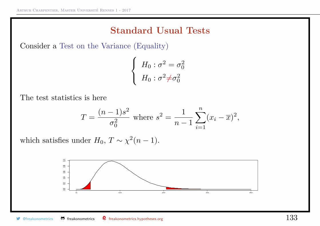
Standard Usual TestsConsider a Test on the Variance (Equality) H0 : σ2 = σ2
0
H0 : σ2 6=σ20
The test statistics is here
T = (n− 1)s2
σ20
where s2 = 1n− 1
n∑i=1
(xi − x)2,
which satisfies under H0, T ∼ χ2(n− 1).
0 10 20 30 40
0.00
0.02
0.04
0.06
0.08
0.10
@freakonometrics freakonometrics freakonometrics.hypotheses.org 133
Arthur Charpentier, Master Université Rennes 1 - 2017
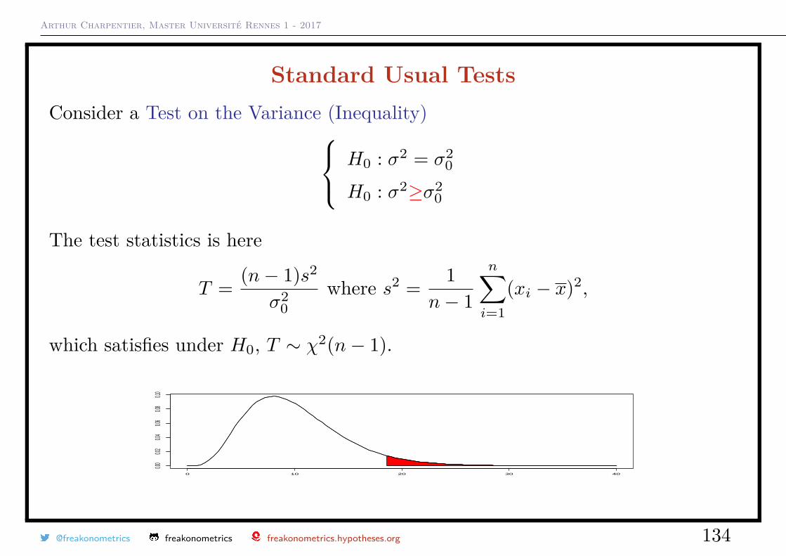
Standard Usual TestsConsider a Test on the Variance (Inequality) H0 : σ2 = σ2
0
H0 : σ2≥σ20
The test statistics is here
T = (n− 1)s2
σ20
where s2 = 1n− 1
n∑i=1
(xi − x)2,
which satisfies under H0, T ∼ χ2(n− 1).
0 10 20 30 40
0.00
0.02
0.04
0.06
0.08
0.10
@freakonometrics freakonometrics freakonometrics.hypotheses.org 134
Arthur Charpentier, Master Université Rennes 1 - 2017
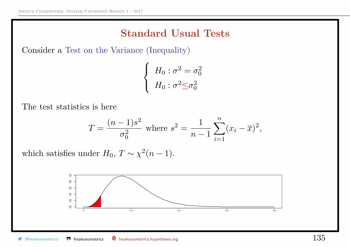
Standard Usual TestsConsider a Test on the Variance (Inequality) H0 : σ2 = σ2
0
H0 : σ2≤σ20
The test statistics is here
T = (n− 1)s2
σ20
where s2 = 1n− 1
n∑i=1
(xi − x)2,
which satisfies under H0, T ∼ χ2(n− 1).
0 10 20 30 40
0.00
0.02
0.04
0.06
0.08
0.10
@freakonometrics freakonometrics freakonometrics.hypotheses.org 135
Arthur Charpentier, Master Université Rennes 1 - 2017
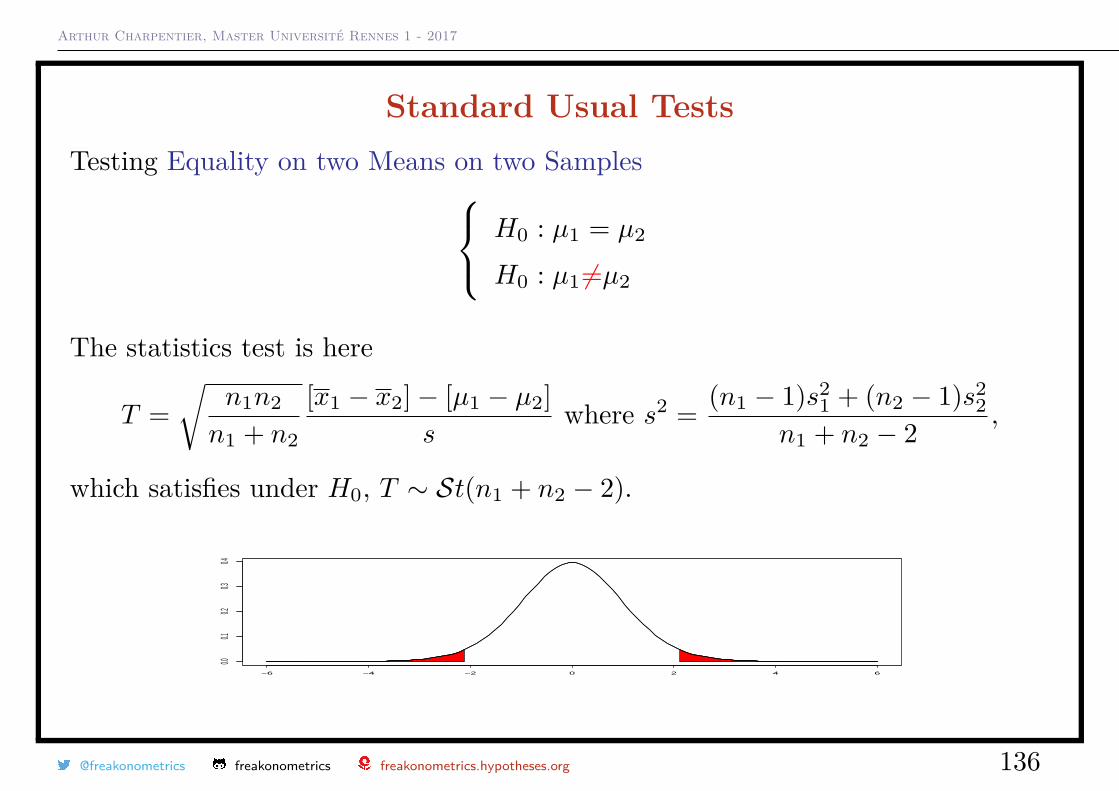
Standard Usual TestsTesting Equality on two Means on two Samples H0 : µ1 = µ2
H0 : µ1 6=µ2
The statistics test is here
T =√
n1n2
n1 + n2
[x1 − x2]− [µ1 − µ2]s
where s2 = (n1 − 1)s21 + (n2 − 1)s2
2n1 + n2 − 2 ,
which satisfies under H0, T ∼ St(n1 + n2 − 2).
−6 −4 −2 0 2 4 6
0.00.1
0.20.3
0.4
@freakonometrics freakonometrics freakonometrics.hypotheses.org 136
Arthur Charpentier, Master Université Rennes 1 - 2017
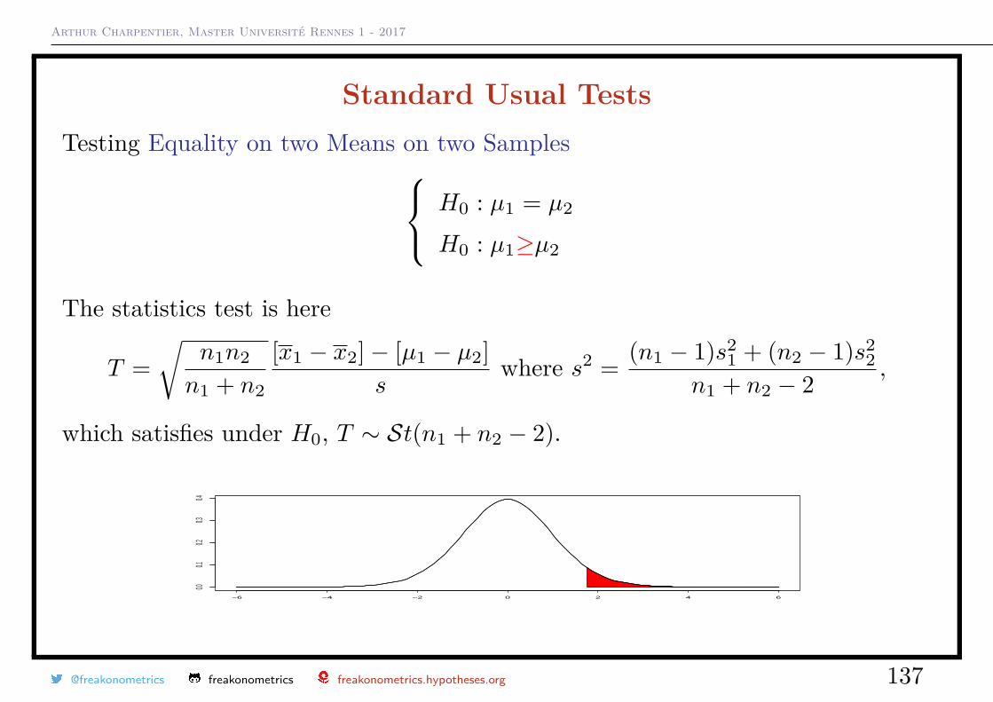
Standard Usual TestsTesting Equality on two Means on two Samples H0 : µ1 = µ2
H0 : µ1≥µ2
The statistics test is here
T =√
n1n2
n1 + n2
[x1 − x2]− [µ1 − µ2]s
where s2 = (n1 − 1)s21 + (n2 − 1)s2
2n1 + n2 − 2 ,
which satisfies under H0, T ∼ St(n1 + n2 − 2).
−6 −4 −2 0 2 4 6
0.00.1
0.20.3
0.4
@freakonometrics freakonometrics freakonometrics.hypotheses.org 137
Arthur Charpentier, Master Université Rennes 1 - 2017
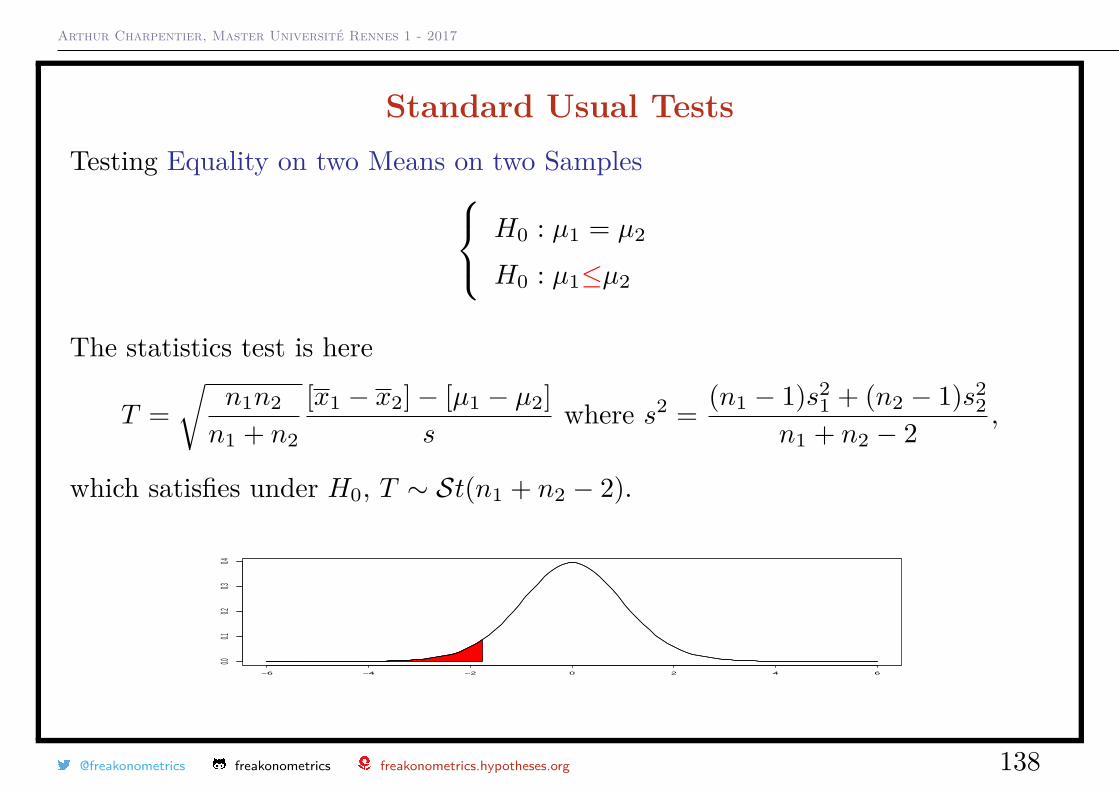
Standard Usual TestsTesting Equality on two Means on two Samples H0 : µ1 = µ2
H0 : µ1≤µ2
The statistics test is here
T =√
n1n2
n1 + n2
[x1 − x2]− [µ1 − µ2]s
where s2 = (n1 − 1)s21 + (n2 − 1)s2
2n1 + n2 − 2 ,
which satisfies under H0, T ∼ St(n1 + n2 − 2).
−6 −4 −2 0 2 4 6
0.00.1
0.20.3
0.4
@freakonometrics freakonometrics freakonometrics.hypotheses.org 138
Arthur Charpentier, Master Université Rennes 1 - 2017
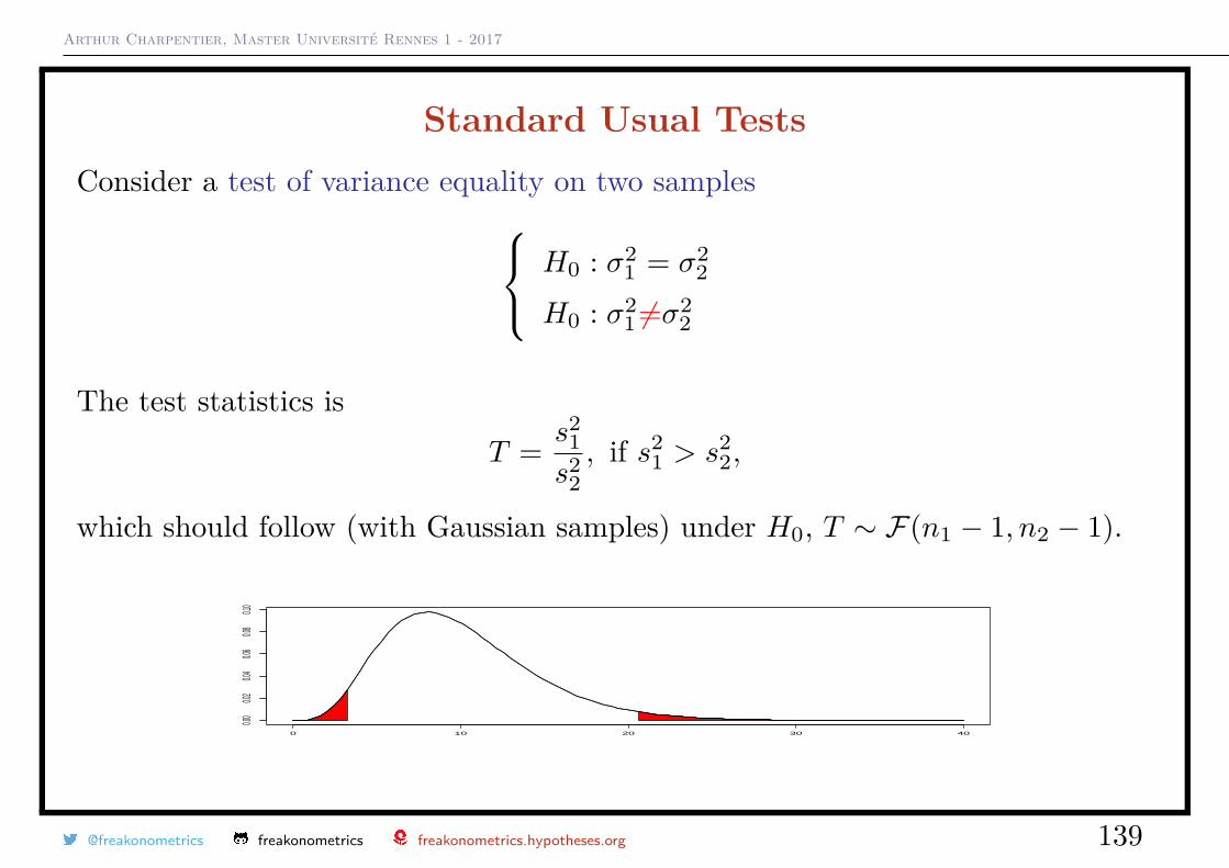
Standard Usual TestsConsider a test of variance equality on two samples H0 : σ2
1 = σ22
H0 : σ21 6=σ2
2
The test statistics isT = s2
1s2
2, if s2
1 > s22,
which should follow (with Gaussian samples) under H0, T ∼ F(n1 − 1, n2 − 1).
0 10 20 30 40
0.00
0.02
0.04
0.06
0.08
0.10
@freakonometrics freakonometrics freakonometrics.hypotheses.org 139
Arthur Charpentier, Master Université Rennes 1 - 2017
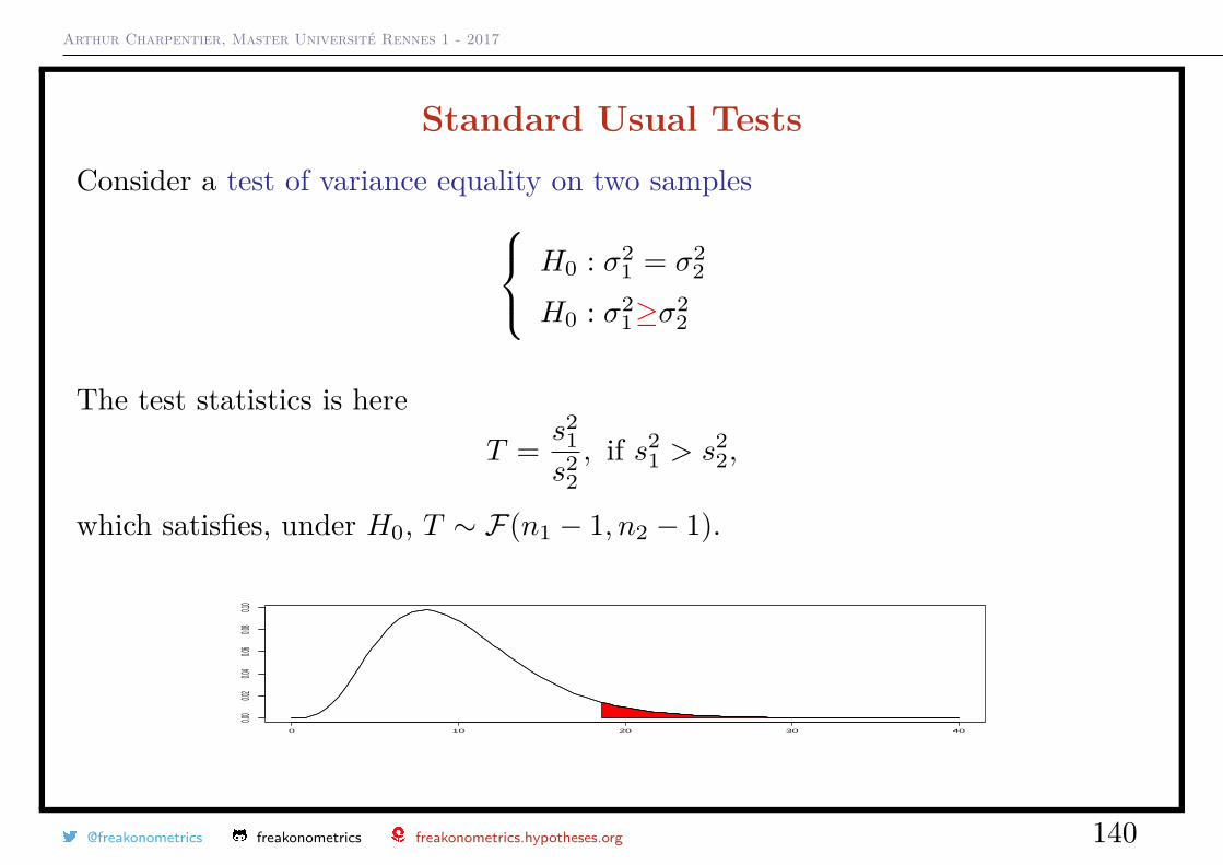
Standard Usual TestsConsider a test of variance equality on two samples H0 : σ2
1 = σ22
H0 : σ21≥σ2
2
The test statistics is hereT = s2
1s2
2, if s2
1 > s22,
which satisfies, under H0, T ∼ F(n1 − 1, n2 − 1).
0 10 20 30 40
0.00
0.02
0.04
0.06
0.08
0.10
@freakonometrics freakonometrics freakonometrics.hypotheses.org 140
Arthur Charpentier, Master Université Rennes 1 - 2017
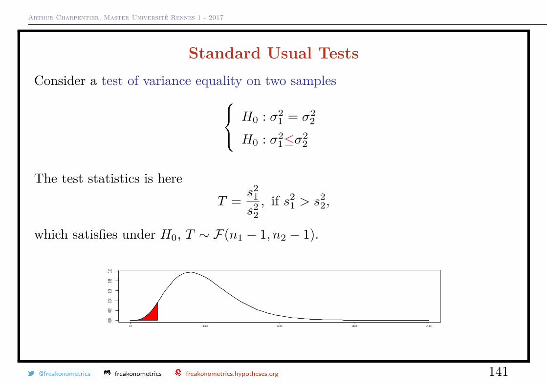
Standard Usual TestsConsider a test of variance equality on two samples H0 : σ2
1 = σ22
H0 : σ21≤σ2
2
The test statistics is hereT = s2
1s2
2, if s2
1 > s22,
which satisfies under H0, T ∼ F(n1 − 1, n2 − 1).
0 10 20 30 40
0.00
0.02
0.04
0.06
0.08
0.10
@freakonometrics freakonometrics freakonometrics.hypotheses.org 141
Arthur Charpentier, Master Université Rennes 1 - 2017
Multinomial TestA multinomial distribution is the natural extension of the binomial distribution,from 2 classes 0, 1 to k classes, say 1, 2, · · · , k.
Let p = (p1, · · · , pk) denote a probability distribution on 1, 2, · · · , k.
For a multinomial distribution, let n denote a vector in Nk such thatn1 + · · ·+ nk = n,
P[N = n] = n!n∏i=1
pniini!
Pearson’s chi-squared test has been introduced to test H0 : p = π againstH1 : p 6= π
X2 =k∑i=1
(ni − nπi)2
nπi
and under H0, X2 ∼ χ2(k − 1).
@freakonometrics freakonometrics freakonometrics.hypotheses.org 142
Arthur Charpentier, Master Université Rennes 1 - 2017
Independence Test (Discrete)This test is based on Pearson’s chi-squared test on the contingency table.
Consider two variables X ∈ 1, 2, · · · , I and Y ∈ 1, 2, · · · , J and let n = [ni,j ]denote the contingency table
ni,j =n∑k=1
1(xk = i, yk = j)
Let ni,· =J∑j=1
ni,j and n·,j =I∑i=1
ni,j .
If variables are independent, ∀i, j
P[x = i, y = j]︸ ︷︷ ︸∼ni,jn
= P[x = i]︸ ︷︷ ︸∼ni,·n
·P[y = j]︸ ︷︷ ︸∼n·,jn
@freakonometrics freakonometrics freakonometrics.hypotheses.org 143
Arthur Charpentier, Master Université Rennes 1 - 2017
Independence Test (Discrete)
Hence, n⊥i,j = ni,·n·,jn
would be the value of the contingency table if variableswere independent.
Here the statistics used to test H0 : X ⊥⊥ Y is
X2 =k∑i=1
(ni,j − n⊥i,j
)2n⊥i,j
and under H0, X2 ∼ χ2([I − 1][J − 1]).
With R, use chisq.test().
@freakonometrics freakonometrics freakonometrics.hypotheses.org 144
Arthur Charpentier, Master Université Rennes 1 - 2017
Independence Test (Continuous)Pearson’s Correlation,
r(X,Y ) = Cov(X,Y )√Var(X)Var(Y )
= E(XY )− E(X)E(Y )√[E(X2)− E(X)2] · [E(Y 2)− E(Y )2]
Spearman’s (Rank) Correlation
ρ(X,Y ) = Cov(FX(X), FY (Y ))√Var(FX(X))Var(FY (Y ))
= 12 Cov(FX(X), FY (Y ))
Let di = Ri − Si = n(FX(xi)− FY (yi)) and define R =∑R2i
Test on Correlation Coefficient
Z = 6R− n(n2 − 1)n(n+ 1)
√n− 1
@freakonometrics freakonometrics freakonometrics.hypotheses.org 145
Arthur Charpentier, Master Université Rennes 1 - 2017
Parametric ModelingConsider a sample x1, · · · , xn, with n independent observations.
Assume that xi’s are obtained from random variables with identical (unknown)distribution F .
In parametric statistics, F belongs to some family F = Fθ;θ ∈ Θ.
• X has a Bernoulli distribution, X ∼ B(p), θ = p ∈ (0, 1),• X has a Poisson distribution, X ∼ P(λ), θ = λ ∈ R+,• X has a Gaussian distribution, X ∼ N (µ, σ), θ = (µ, σ) ∈ R× R+,
We want to find the best choice for θ, the true unknown value of the parameter,so that X ∼ Fθ.
@freakonometrics freakonometrics freakonometrics.hypotheses.org 146
Arthur Charpentier, Master Université Rennes 1 - 2017
Heads and TailsConsider the following sample
head,head, tail,head, tail,head, tail, tail,head, tail,head, tail
that we will convert using
X =
1 if head0 if tail.
Our sampleis now1, 1, 0, 1, 0, 1, 0, 0, 1, 0, 1, 0
Here X has a Bernoulli distribution X ∼ B(p), where parameter p is unknown.
@freakonometrics freakonometrics freakonometrics.hypotheses.org 147
Arthur Charpentier, Master Université Rennes 1 - 2017
Statistical InferenceWhat is the true unknown value of p ?
• What is the value for p that could be the most likely?
Over n draws, the probability to get exactly our sample x1, · · · , xn is
P(X1 = x1, · · · , Xn = xn),
where X1, · · · , Xn are n independent verions of X, with distribution B(p). Hence,
P(X1 = x1, · · · , Xn = xn) =n∏i=1
P(Xi = xi) =n∏i=1
pxi × (1− p)1−xi ,
because pxi × (1− p)1−xi =
p if xi equals 11− p if xi equals 0
@freakonometrics freakonometrics freakonometrics.hypotheses.org 148
Arthur Charpentier, Master Université Rennes 1 - 2017
Statistical InferenceThus,
P(X1 = x1, · · · , Xn = xn) = p∑n
i=1xi × (1− p)
∑n
i=11−xi .
This function which depends on p (but also x1, · · · , xn) is called likelihood ofthe sample, and is denoted L,
L(p;x1, · · · , xn) = p∑n
i=1xi × (1− p)
∑n
i=11−xi .
Here we have obtained 5 times 1’s and 6 times 0’s. As a function of p we get thedifference likelihoods,
@freakonometrics freakonometrics freakonometrics.hypotheses.org 149
Arthur Charpentier, Master Université Rennes 1 - 2017
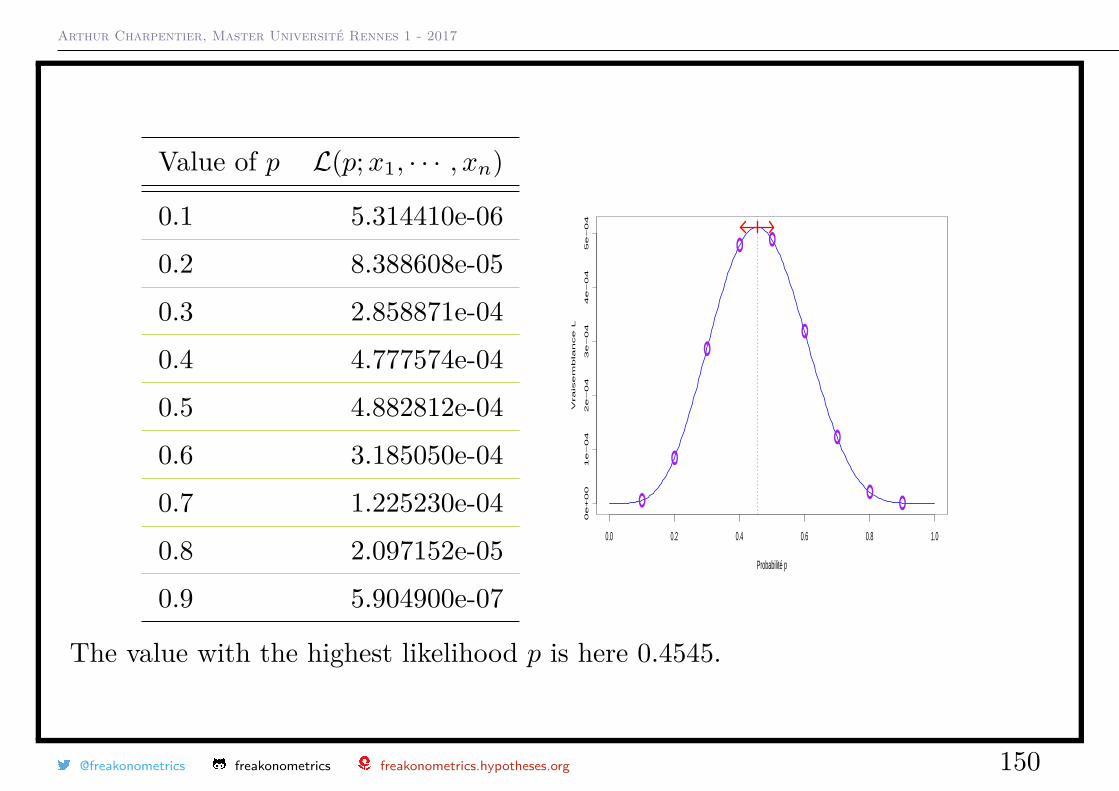
Value of p L(p;x1, · · · , xn)
0.1 5.314410e-06
0.2 8.388608e-05
0.3 2.858871e-04
0.4 4.777574e-04
0.5 4.882812e-04
0.6 3.185050e-04
0.7 1.225230e-04
0.8 2.097152e-05
0.9 5.904900e-07
0.0 0.2 0.4 0.6 0.8 1.0
0e
+0
01
e−
04
2e
−0
43
e−
04
4e
−0
45
e−
04
Probabilité pV
ra
ise
mb
lan
ce
L
The value with the highest likelihood p is here 0.4545.
@freakonometrics freakonometrics freakonometrics.hypotheses.org 150
Arthur Charpentier, Master Université Rennes 1 - 2017
Statistical Inference
• Why not use the (empirical) mean?
We have obtained the following sample
1, 1, 0, 1, 0, 1, 0, 0, 1, 0, 1, 0
For a Bernoulli distribution, E(X) = p. Thus, it can be seen as natural to use aestimator of p an estimator of E(X), the average of 1’s is our sample, x.
A natural estimator for p would be x 5/11 = 0.4545.
@freakonometrics freakonometrics freakonometrics.hypotheses.org 151
Arthur Charpentier, Master Université Rennes 1 - 2017
Maximum LikelihoodIn a more general setting, let fθ denote the true (unknown) distribution of X,
• if X is continuous, fθ denotes the density i.e. fθ(x) = dF (x)dx
= F ′(x),• if X is discrete, fθ denotes the probability fθ(x) = P(X = x),
Since Xi’s are i.i.d., the likelihood of the sample is
L(θ;x1, · · · , xn) = P(X1 = x1, · · · , Xn = xn) =n∏i=1
fθ(xi)
A natural estimator for θ is obtained as the maximum of the likelihood
θ ∈ argmaxL(θ;x1, · · · , xn),θ ∈ Θ.
One should keep in mind that for any increasing function h,
θ ∈ argmaxh (L(θ;x1, · · · , xn)) ,θ ∈ Θ.
@freakonometrics freakonometrics freakonometrics.hypotheses.org 152
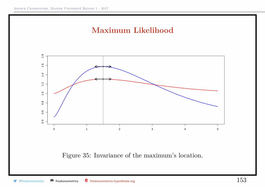
Arthur Charpentier, Master Université Rennes 1 - 2017
Maximum Likelihood
0 1 2 3 4 5
0.4
0.6
0.8
1.0
1.2
1.4
1.6
1.8
Figure 35: Invariance of the maximum’s location.
@freakonometrics freakonometrics freakonometrics.hypotheses.org 153
Arthur Charpentier, Master Université Rennes 1 - 2017
Maximum LikelihoodConsider the case here where h = log
θ ∈ argmaxlog (L(θ;x1, · · · , xn)) ,θ ∈ Θ.
i.e. equivalently, we can look for the maximum of the log-likelihood, which can bewritten
logL(θ;x1, · · · , xn) =n∑i=1
log fθ(xi)
From a practical perspective, the first order condition will ask us to computederivatives, and the derivative of a sum is easier to derive than the derivative of aproduct, assuming that θ → L(θ;x) is differentiable.
@freakonometrics freakonometrics freakonometrics.hypotheses.org 154
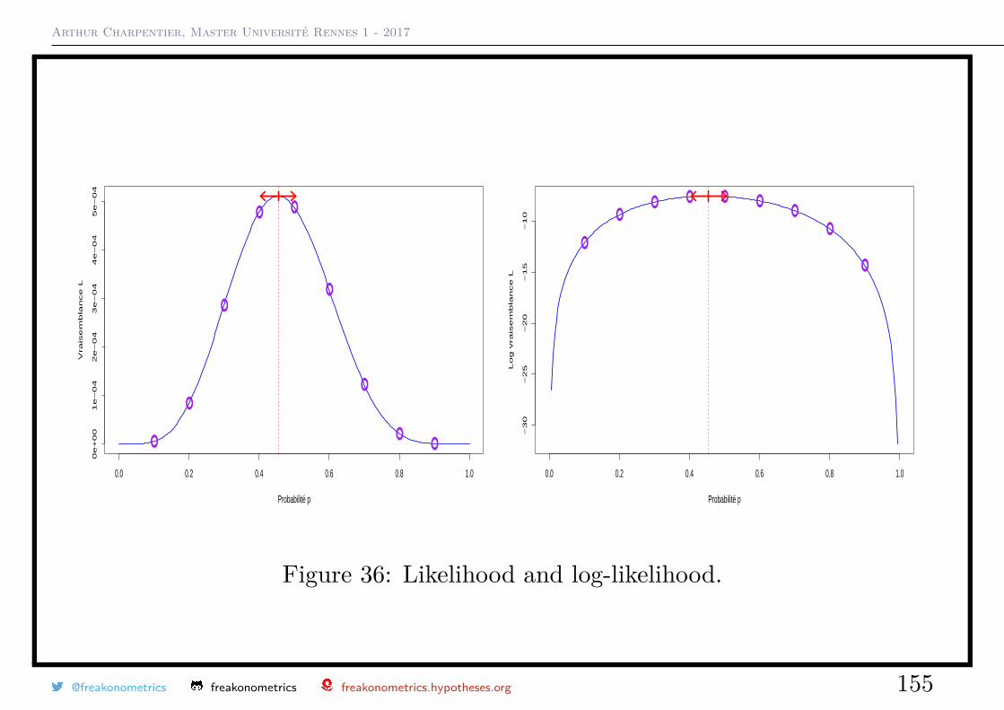
Arthur Charpentier, Master Université Rennes 1 - 2017
0.0 0.2 0.4 0.6 0.8 1.0
0e
+0
01
e−
04
2e
−0
43
e−
04
4e
−0
45
e−
04
Probabilité p
Vra
ise
mb
lan
ce
L
0.0 0.2 0.4 0.6 0.8 1.0
−3
0−
25
−2
0−
15
−1
0
Probabilité pL
og
vra
ise
mb
lan
ce
L
Figure 36: Likelihood and log-likelihood.
@freakonometrics freakonometrics freakonometrics.hypotheses.org 155
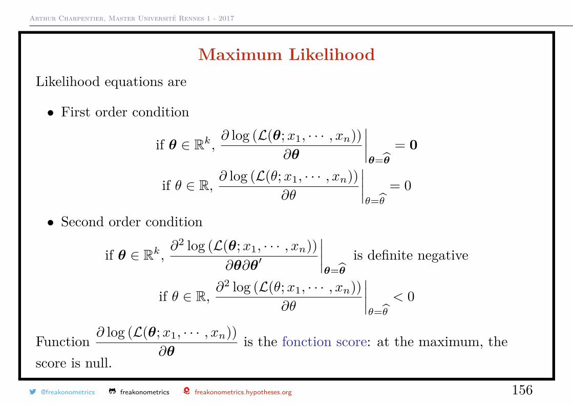
Arthur Charpentier, Master Université Rennes 1 - 2017
Maximum LikelihoodLikelihood equations are
• First order condition
if θ ∈ Rk,∂ log (L(θ;x1, · · · , xn))
∂θ
∣∣∣∣θ=θ
= 0
if θ ∈ R,∂ log (L(θ;x1, · · · , xn))
∂θ
∣∣∣∣θ=θ
= 0
• Second order condition
if θ ∈ Rk,∂2 log (L(θ;x1, · · · , xn))
∂θ∂θ′
∣∣∣∣θ=θ
is definite negative
if θ ∈ R,∂2 log (L(θ;x1, · · · , xn))
∂θ
∣∣∣∣θ=θ
< 0
Function ∂ log (L(θ;x1, · · · , xn))∂θ
is the fonction score: at the maximum, thescore is null.
@freakonometrics freakonometrics freakonometrics.hypotheses.org 156
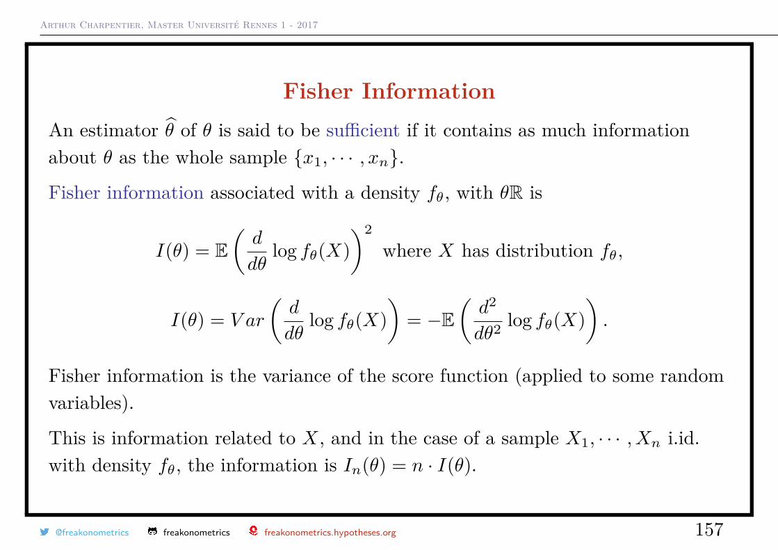
Arthur Charpentier, Master Université Rennes 1 - 2017
Fisher InformationAn estimator θ of θ is said to be sufficient if it contains as much informationabout θ as the whole sample x1, · · · , xn.
Fisher information associated with a density fθ, with θR is
I(θ) = E(d
dθlog fθ(X)
)2where X has distribution fθ,
I(θ) = V ar
(d
dθlog fθ(X)
)= −E
(d2
dθ2 log fθ(X)).
Fisher information is the variance of the score function (applied to some randomvariables).
This is information related to X, and in the case of a sample X1, · · · , Xn i.id.with density fθ, the information is In(θ) = n · I(θ).
@freakonometrics freakonometrics freakonometrics.hypotheses.org 157
Arthur Charpentier, Master Université Rennes 1 - 2017
Efficiency and Optimality
If θ is an unbiased estimator of θ, then Var(θ) ≥ 1nI(θ) . If that bound is
attained, the estimator is said to beefficient.
Note that this lower bound is not necessarily reached.
An unbiased estimator θ is said to be optimal if it has the lowest variance amongall unbiased estimators.
Fisher information in higher dimensionIf θ ∈ Rk, then Fisher information is the k × k matrix I = [Ii,j ] with
Ii,j = E(∂
∂θilog fθ(X) ∂
∂θjlog fθ(X)
).
@freakonometrics freakonometrics freakonometrics.hypotheses.org 158
Arthur Charpentier, Master Université Rennes 1 - 2017
Fisher Information & ComputationsAssume that X has a Poisson distribution P(θ),
log fθ(x) = −θ + x log θ − log(x!) and d2
dθ2 log fθ(x) = − x
θ2
I(θ) = −E(d2
dθ2 log fθ(X))
= −E(−Xθ2
)= 1θ
For a binomial distribution B(n, θ), I(θ) = n
θ(1− θ)
For a Gaussian distribution N (θ, σ2), I(θ) = 1σ2
For a Gaussian distribution N (µ, θ), I(θ) = 12θ2
@freakonometrics freakonometrics freakonometrics.hypotheses.org 159
Arthur Charpentier, Master Université Rennes 1 - 2017
Maximum LikelihoodDefinition Let x1, · · · , xn be a sample with distribution fθ, where θ ∈ Θ.The maximum likelihood estimator θn of θ is
θn ∈ argmaxL(θ;x1, · · · , xn),θ ∈ Θ
.
Proposition. Under some technical assumptions θn converges almost surelytowards θ, θn
a.s.→ θ, as n→∞.Proposition. Under some technical assumptions θn is asymptotically efficient,
√n(θn − θ) L→ N (0, I−1(θ)).
Results are only asymptotic, there is no reason, e.g., to have an unbiasedestimator.
@freakonometrics freakonometrics freakonometrics.hypotheses.org 160
Arthur Charpentier, Master Université Rennes 1 - 2017
Gaussian case, N (µ, σ2)Let x1, · · · , xn be a sample from a N (µ, σ2) distribution, with density
f(x | µ, σ2) = 1√2π σ
exp(− (x− µ)2
2σ2
).
The likelihood is here
f(x1, . . . , xn | µ, σ2) =n∏i=1
f(xi | µ, σ2) =(
12πσ2
)n/2exp
(−∑ni=1(xi − µ)2
2σ2
),
i.e.
L(µ, σ2) =(
12πσ2
)n/2exp
(−∑ni=1(xi − x)2 + n(x− µ)2
2σ2
).
@freakonometrics freakonometrics freakonometrics.hypotheses.org 161
Arthur Charpentier, Master Université Rennes 1 - 2017
Gaussian case, N (µ, σ2)The maximum likelihood estimator of µ is obtained from the first order equations
∂
∂µlogL
= ∂
∂µlog((
12πσ2
)n/2exp
(−∑ni=1(xi − x)2 + n(x− µ)2
2σ2
))
= ∂
∂µ
(log(
12πσ2
)n/2−∑ni=1(xi − x)2 + n(x− µ)2
2σ2
)
= 0− −2n(x− µ)2σ2 = 0.
i.e. µ = x = 1n
n∑i=1
xi.
@freakonometrics freakonometrics freakonometrics.hypotheses.org 162
Arthur Charpentier, Master Université Rennes 1 - 2017
The second part of the first order condition is here
∂
∂σlog((
12πσ2
)n/2exp
(−∑ni=1(xi − x)2 + n(x− µ)2
2σ2
))
= ∂
∂σ
(n
2 log(
12πσ2
)−∑ni=1(xi − x)2 + n(x− µ)2
2σ2
)= −n
σ+∑ni=1(xi − x)2 + n(x− µ)2
σ3 = 0.
The first order condition yields
σ2 = 1n
n∑i=1
(xi − µ)2 = 1n
n∑i=1
(xi − x)2 = 1n
n∑i=1
x2i −
1n2
n∑i=1
n∑j=1
xixj .
Observe that here E [µ] = µ, while E[σ2] 6= σ2.
@freakonometrics freakonometrics freakonometrics.hypotheses.org 163
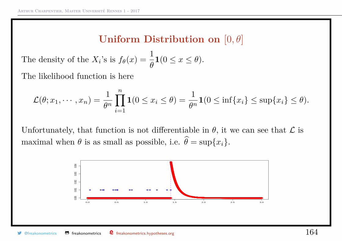
Arthur Charpentier, Master Université Rennes 1 - 2017
Uniform Distribution on [0, θ]
The density of the Xi’s is fθ(x) = 1θ1(0 ≤ x ≤ θ).
The likelihood function is here
L(θ;x1, · · · , xn) = 1θn
n∏i=1
1(0 ≤ xi ≤ θ) = 1θn
1(0 ≤ infxi ≤ supxi ≤ θ).
Unfortunately, that function is not differentiable in θ, it we can see that L ismaximal when θ is as small as possible, i.e. θ = supxi.
0.0 0.5 1.0 1.5 2.0 2.5 3.0
0.000
0.001
0.002
0.003
0.004
@freakonometrics freakonometrics freakonometrics.hypotheses.org 164

Arthur Charpentier, Master Université Rennes 1 - 2017
Uniform Distribution on [θ, θ + 1]In some case, the maximum likelihood is not unique.
Assume that x1, · · · , xn are uniformly distributed on [θ, θ + 1]. If
θ− = supxi − 1 < infxi = θ+
then any estimator θ ∈ [θ−, θ+] is a maximum likelihood estimator of θ.
And as mentioned already, the maximum likelihood estimator is not necessairlyunbiased. For the exponential distribution, θ = 1/x. One can prove that in thatcase
E(θ) = n
n− 1θ > θ.
@freakonometrics freakonometrics freakonometrics.hypotheses.org 165
Arthur Charpentier, Master Université Rennes 1 - 2017
Numerical AspectsFor standard distribution, in R, use library(MASS) to get the maximum likelihoodestimator, e.g. fitdistr(x.norm,"normal") for a normal distribution and a sample x.
One can also use numerical algorithm, in R. It is necessary to define thelog-likelihood LV <- function(theta)-sum(log(dexp(x,theta))) and the useoptim(2,LV) to get the minimum of that function (since it computes a minimum,use the opposite of the log-likelihood).
Numerically, those function are based on Newton-Rahpson also called Fisher’sscore to approximate the maximum of that function.
Let S(x, θ) = ∂
∂θlog f(x, θ) the score function. Set
Sn(θ) =n∑i=1
S(Xi, θ).
@freakonometrics freakonometrics freakonometrics.hypotheses.org 166
Arthur Charpentier, Master Université Rennes 1 - 2017
Numerical AspectsThen use Taylor approximation of Sn in the neighbourhood of θ0,
Sn(x) = Sn(θ0) + (x− θ0)S′n(y) for some y ∈ [x, θ0]
Set x = θn, then
Sn(θn) = 0 = +(θn − θ0)S′n(y) for some y ∈ [θ0, θn]
Hence, θn = θ0 −Sn(θ0)S′n(y) for y ∈ [θ0, θn]
@freakonometrics freakonometrics freakonometrics.hypotheses.org 167
Arthur Charpentier, Master Université Rennes 1 - 2017
Numerical AspectsLet us now construct the following sequence (Newton-Raphson)
θ(i+1)n = θ(i)
n −Sn(θ(i)
n )S′n(θ(i)
n ),
from some starting value θ(0)n (hopefully well chosen).
This can be seen as the Score technique
θ(i+1)n = θ(i)
n −Sn(θ(i)
n )nI(θ(i)
n ),
again from some starting value.
@freakonometrics freakonometrics freakonometrics.hypotheses.org 168
Arthur Charpentier, Master Université Rennes 1 - 2017
Testing Procedures Based on Maximum LikelihoodConsider the heads/tails problem.
We can derive an asyptotic confidence interval from properties of the maximumlikelihood √
n(π − π) L→ N (0, I−1(π))
where I(π) denotes Fisher’s information, i.e.
I(π) = 1π[1− π]
which yields the following (95%) confidence interval for π[π ± 1.96√
n
√π[1− π]
].
@freakonometrics freakonometrics freakonometrics.hypotheses.org 169
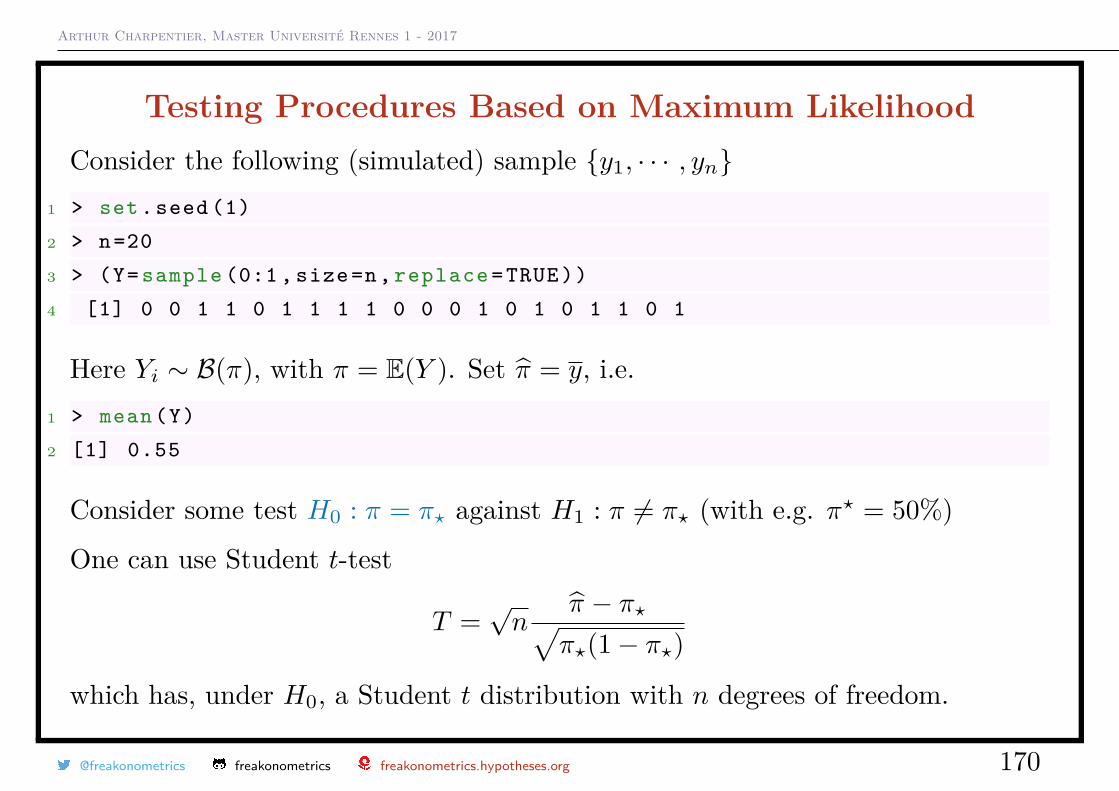
Arthur Charpentier, Master Université Rennes 1 - 2017
Testing Procedures Based on Maximum LikelihoodConsider the following (simulated) sample y1, · · · , yn
1 > set.seed (1)
2 > n=20
3 > (Y= sample (0:1 , size=n, replace =TRUE))
4 [1] 0 0 1 1 0 1 1 1 1 0 0 0 1 0 1 0 1 1 0 1
Here Yi ∼ B(π), with π = E(Y ). Set π = y, i.e.1 > mean(Y)
2 [1] 0.55
Consider some test H0 : π = π? against H1 : π 6= π? (with e.g. π? = 50%)
One can use Student t-test
T =√n
π − π?√π?(1− π?)
which has, under H0, a Student t distribution with n degrees of freedom.
@freakonometrics freakonometrics freakonometrics.hypotheses.org 170
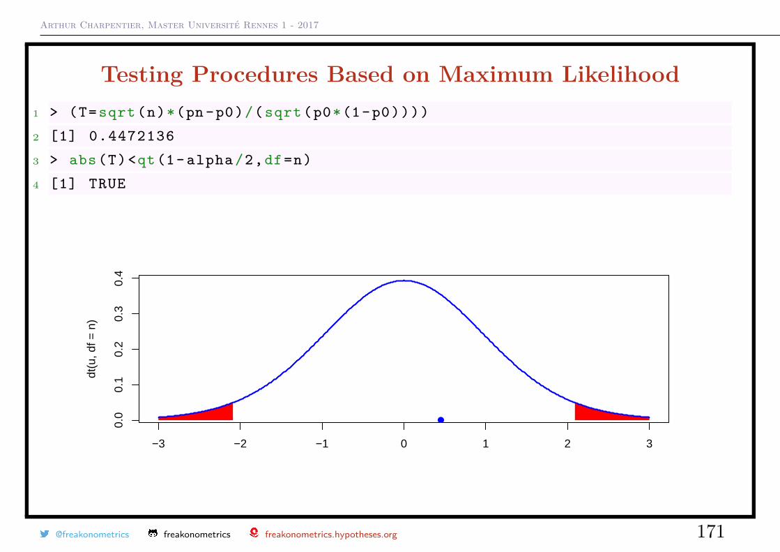
Arthur Charpentier, Master Université Rennes 1 - 2017
Testing Procedures Based on Maximum Likelihood1 > (T=sqrt(n)*(pn -p0)/(sqrt(p0*(1-p0))))
2 [1] 0.4472136
3 > abs(T)<qt(1- alpha /2,df=n)
4 [1] TRUE
−3 −2 −1 0 1 2 3
0.0
0.1
0.2
0.3
0.4
dt(u
, df =
n)
@freakonometrics freakonometrics freakonometrics.hypotheses.org 171
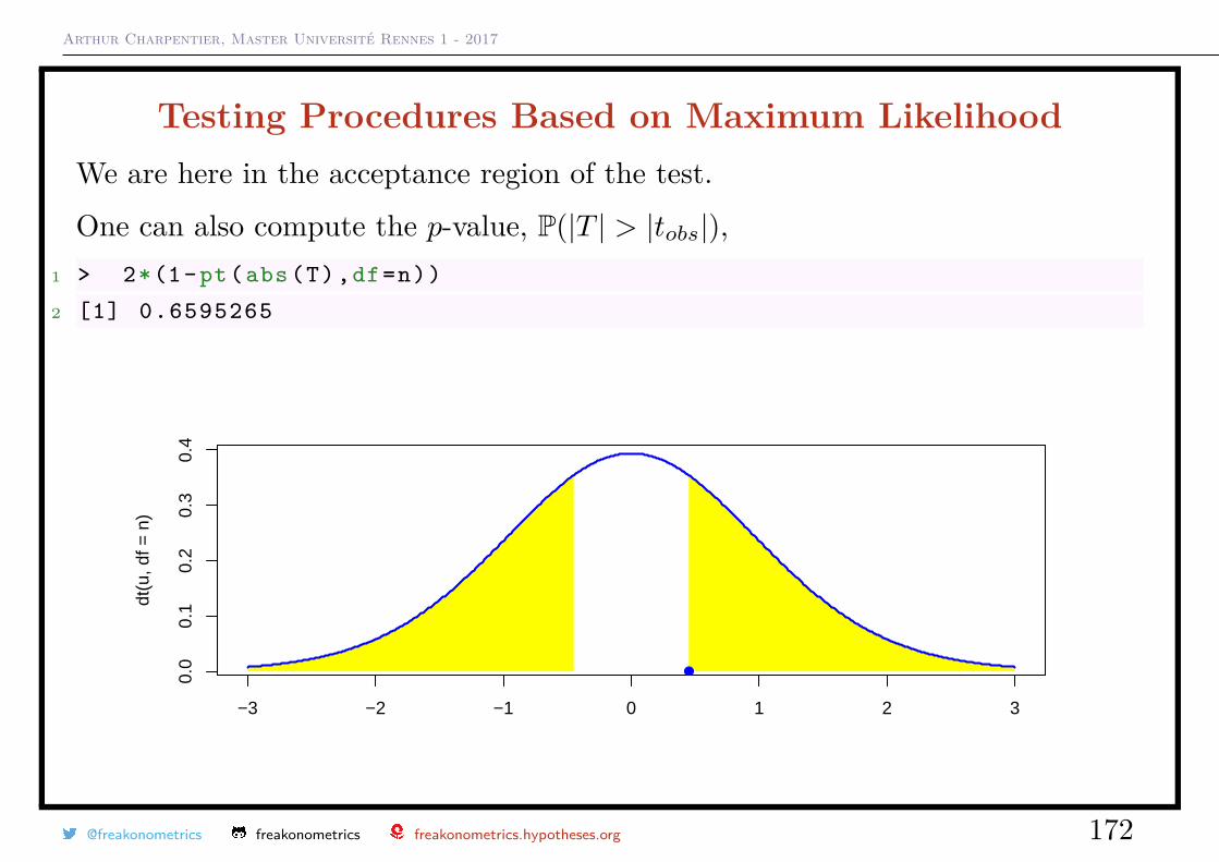
Arthur Charpentier, Master Université Rennes 1 - 2017
Testing Procedures Based on Maximum LikelihoodWe are here in the acceptance region of the test.
One can also compute the p-value, P(|T | > |tobs|),1 > 2*(1-pt(abs(T),df=n))
2 [1] 0.6595265
−3 −2 −1 0 1 2 3
0.0
0.1
0.2
0.3
0.4
dt(u
, df =
n)
@freakonometrics freakonometrics freakonometrics.hypotheses.org 172
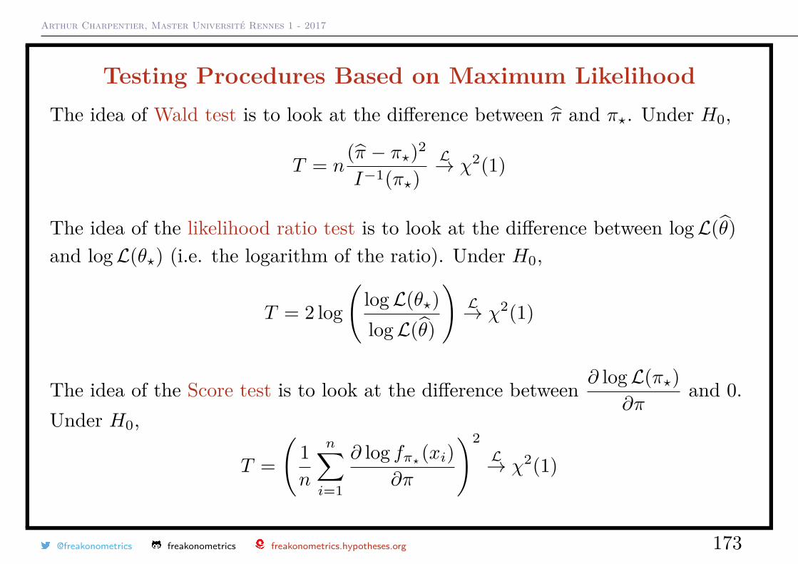
Arthur Charpentier, Master Université Rennes 1 - 2017
Testing Procedures Based on Maximum LikelihoodThe idea of Wald test is to look at the difference between π and π?. Under H0,
T = n(π − π?)2
I−1(π?)L→ χ2(1)
The idea of the likelihood ratio test is to look at the difference between logL(θ)and logL(θ?) (i.e. the logarithm of the ratio). Under H0,
T = 2 log(
logL(θ?)logL(θ)
)L→ χ2(1)
The idea of the Score test is to look at the difference between ∂ logL(π?)∂π
and 0.Under H0,
T =(
1n
n∑i=1
∂ log fπ?(xi)∂π
)2L→ χ2(1)
@freakonometrics freakonometrics freakonometrics.hypotheses.org 173
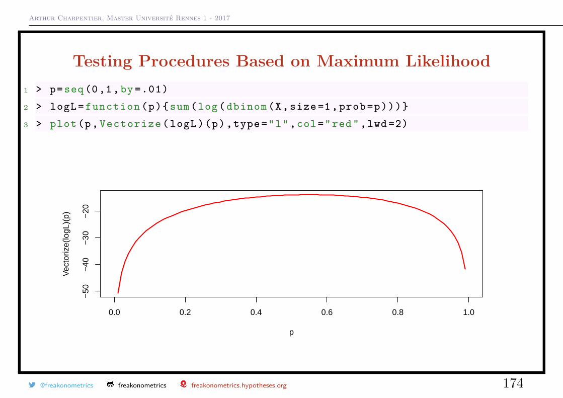
Arthur Charpentier, Master Université Rennes 1 - 2017
Testing Procedures Based on Maximum Likelihood1 > p=seq (0,1,by =.01)
2 > logL= function (p)sum(log( dbinom (X,size =1, prob=p)))
3 > plot(p, Vectorize (logL)(p),type="l",col="red",lwd =2)
0.0 0.2 0.4 0.6 0.8 1.0
−50
−40
−30
−20
p
Vec
toriz
e(lo
gL)(
p)
@freakonometrics freakonometrics freakonometrics.hypotheses.org 174
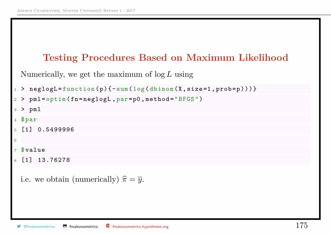
Arthur Charpentier, Master Université Rennes 1 - 2017
Testing Procedures Based on Maximum LikelihoodNumerically, we get the maximum of logL using
1 > neglogL = function (p)-sum(log( dbinom (X,size =1, prob=p)))
2 > pml= optim (fn=neglogL ,par=p0 , method ="BFGS")
3 > pml
4 $par
5 [1] 0.5499996
6
7 $ value
8 [1] 13.76278
i.e. we obtain (numerically) π = y.
@freakonometrics freakonometrics freakonometrics.hypotheses.org 175
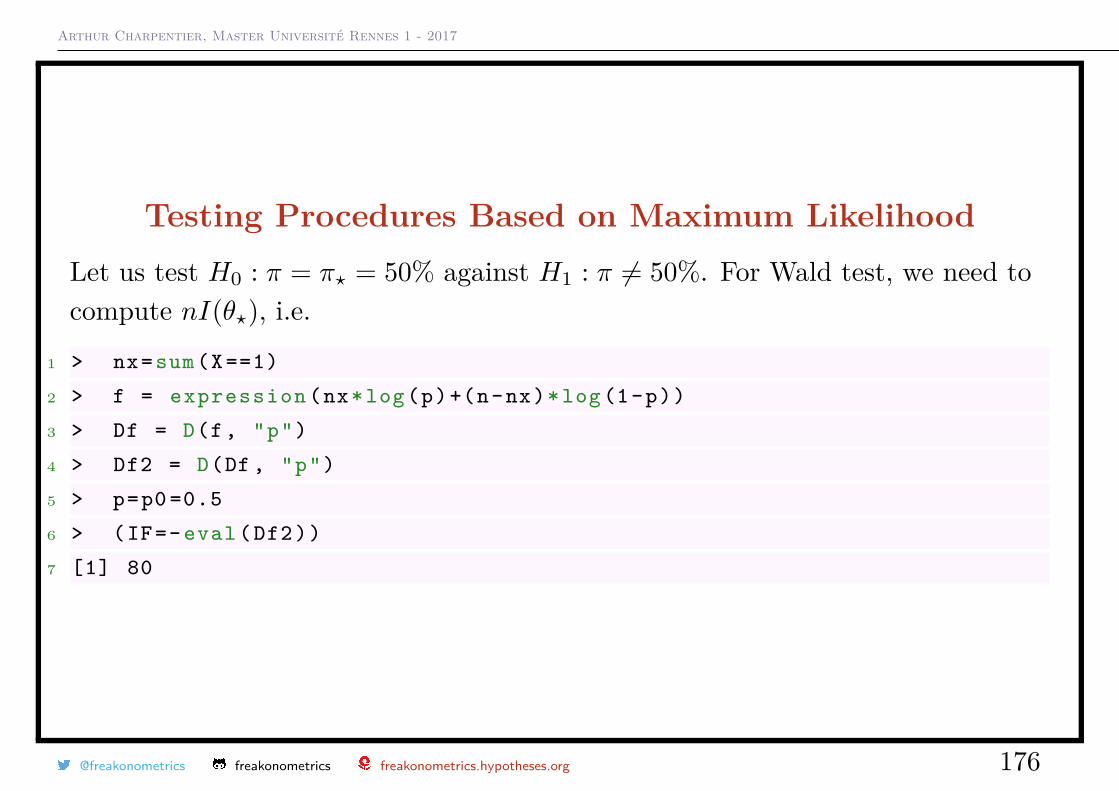
Arthur Charpentier, Master Université Rennes 1 - 2017
Testing Procedures Based on Maximum LikelihoodLet us test H0 : π = π? = 50% against H1 : π 6= 50%. For Wald test, we need tocompute nI(θ?), i.e.
1 > nx=sum(X==1)
2 > f = expression (nx*log(p)+(n-nx)*log (1-p))
3 > Df = D(f, "p")
4 > Df2 = D(Df , "p")
5 > p=p0 =0.5
6 > (IF=-eval(Df2))
7 [1] 80
@freakonometrics freakonometrics freakonometrics.hypotheses.org 176
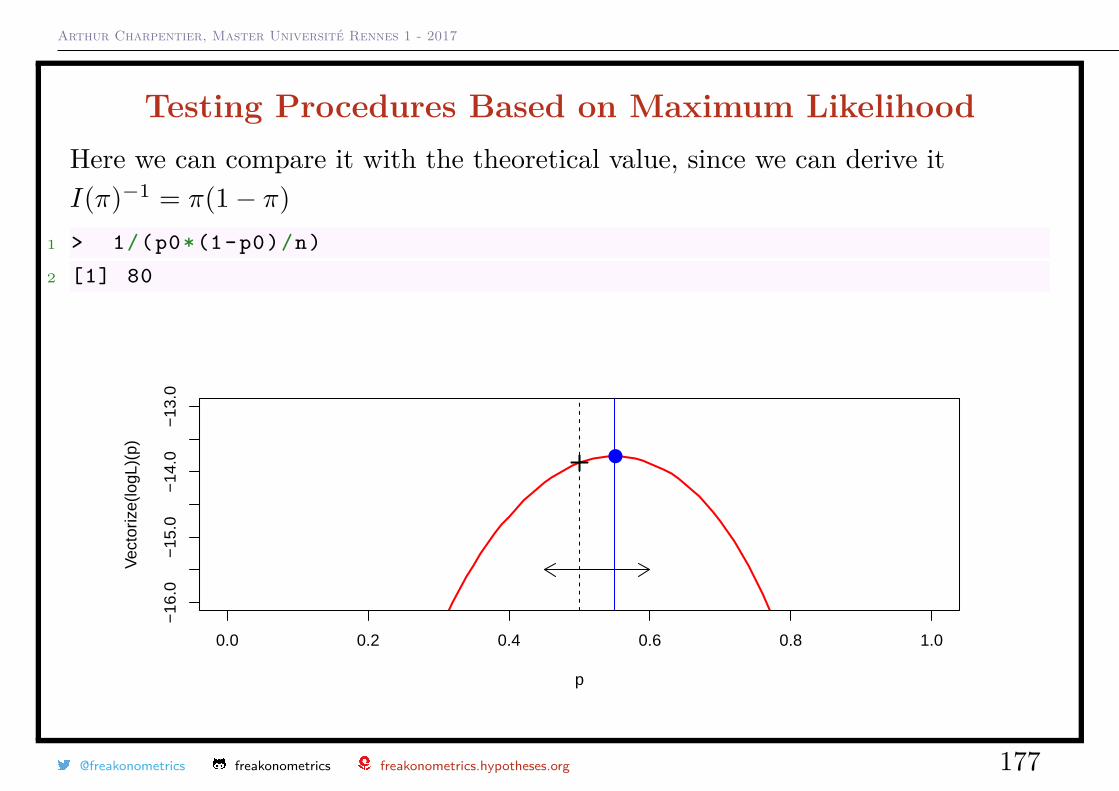
Arthur Charpentier, Master Université Rennes 1 - 2017
Testing Procedures Based on Maximum LikelihoodHere we can compare it with the theoretical value, since we can derive itI(π)−1 = π(1− π)
1 > 1/(p0*(1-p0)/n)
2 [1] 80
0.0 0.2 0.4 0.6 0.8 1.0
−16
.0−
15.0
−14
.0−
13.0
p
Vec
toriz
e(lo
gL)(
p)
@freakonometrics freakonometrics freakonometrics.hypotheses.org 177
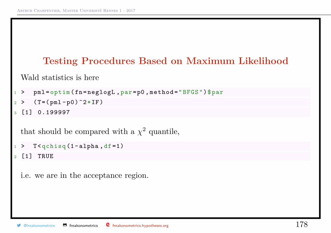
Arthur Charpentier, Master Université Rennes 1 - 2017
Testing Procedures Based on Maximum LikelihoodWald statistics is here
1 > pml= optim (fn=neglogL ,par=p0 , method ="BFGS")$par
2 > (T=(pml -p0)^2*IF)
3 [1] 0.199997
that should be compared with a χ2 quantile,1 > T< qchisq (1-alpha ,df =1)
2 [1] TRUE
i.e. we are in the acceptance region.
@freakonometrics freakonometrics freakonometrics.hypotheses.org 178
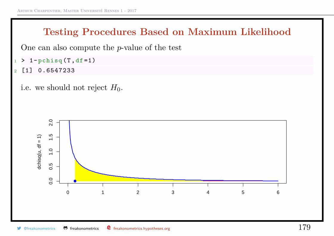
Arthur Charpentier, Master Université Rennes 1 - 2017
Testing Procedures Based on Maximum LikelihoodOne can also compute the p-value of the test
1 > 1- pchisq (T,df =1)
2 [1] 0.6547233
i.e. we should not reject H0.
0 1 2 3 4 5 6
0.0
0.5
1.0
1.5
2.0
dchi
sq(u
, df =
1)
@freakonometrics freakonometrics freakonometrics.hypotheses.org 179
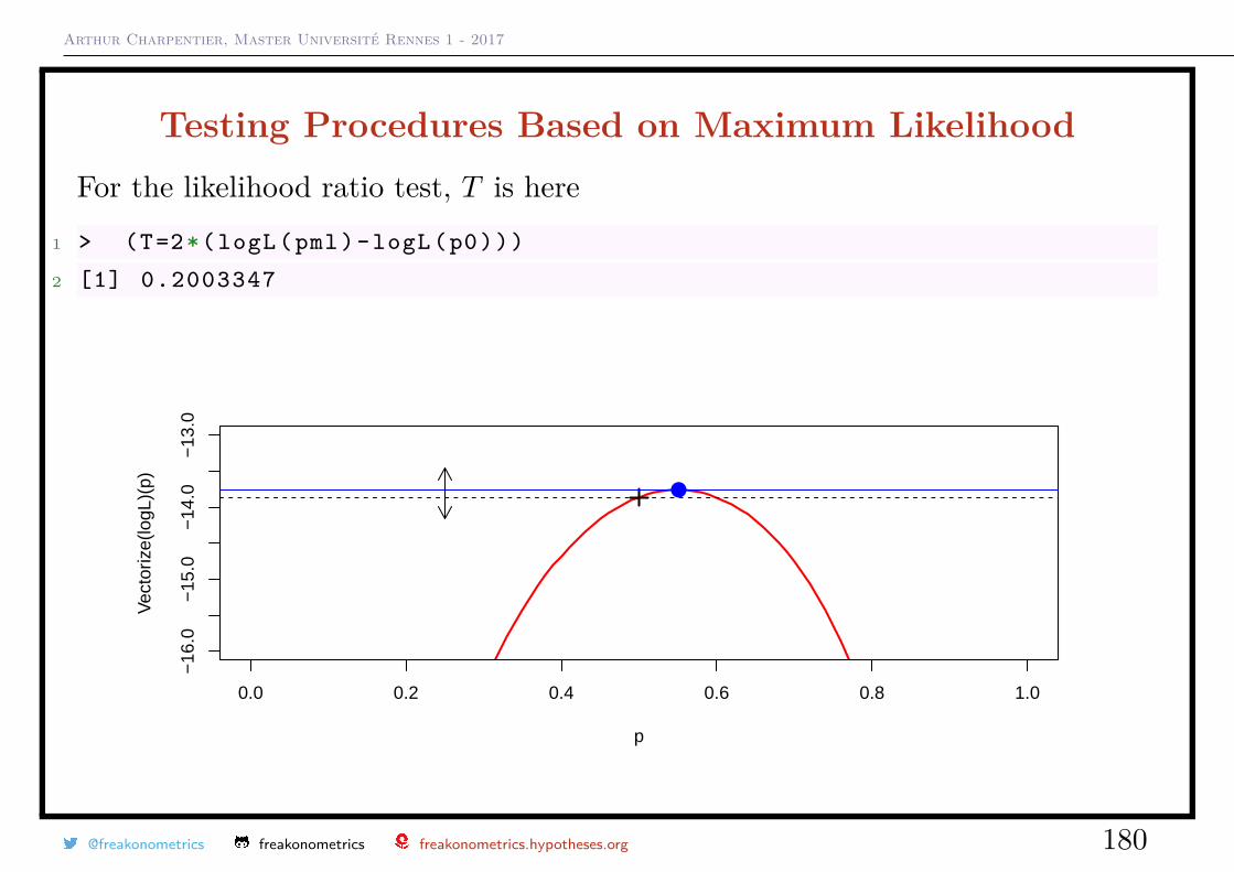
Arthur Charpentier, Master Université Rennes 1 - 2017
Testing Procedures Based on Maximum LikelihoodFor the likelihood ratio test, T is here
1 > (T=2*(logL(pml)-logL(p0)))
2 [1] 0.2003347
0.0 0.2 0.4 0.6 0.8 1.0
−16
.0−
15.0
−14
.0−
13.0
p
Vec
toriz
e(lo
gL)(
p)
@freakonometrics freakonometrics freakonometrics.hypotheses.org 180
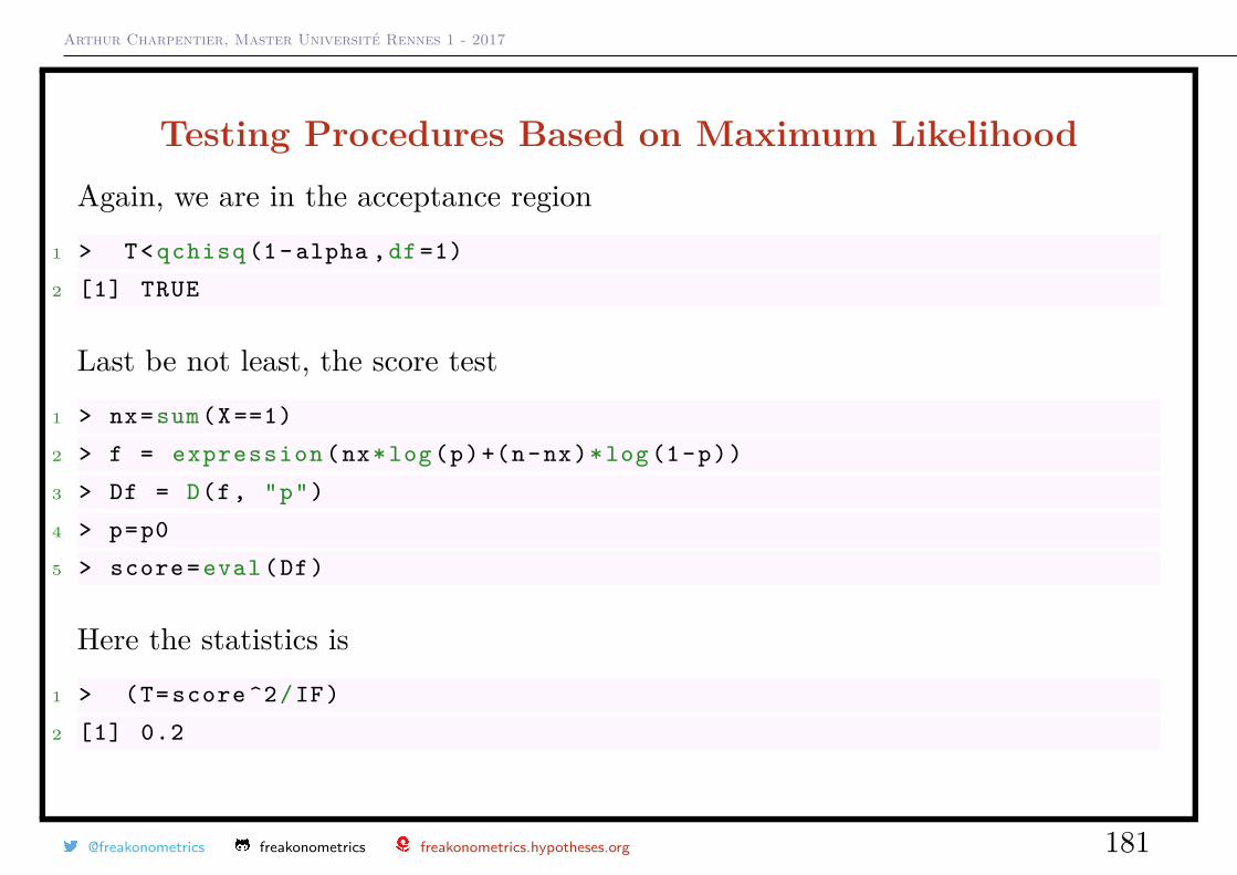
Arthur Charpentier, Master Université Rennes 1 - 2017
Testing Procedures Based on Maximum LikelihoodAgain, we are in the acceptance region
1 > T< qchisq (1-alpha ,df =1)
2 [1] TRUE
Last be not least, the score test1 > nx=sum(X==1)
2 > f = expression (nx*log(p)+(n-nx)*log (1-p))
3 > Df = D(f, "p")
4 > p=p0
5 > score =eval(Df)
Here the statistics is1 > (T= score ^2/IF)
2 [1] 0.2
@freakonometrics freakonometrics freakonometrics.hypotheses.org 181
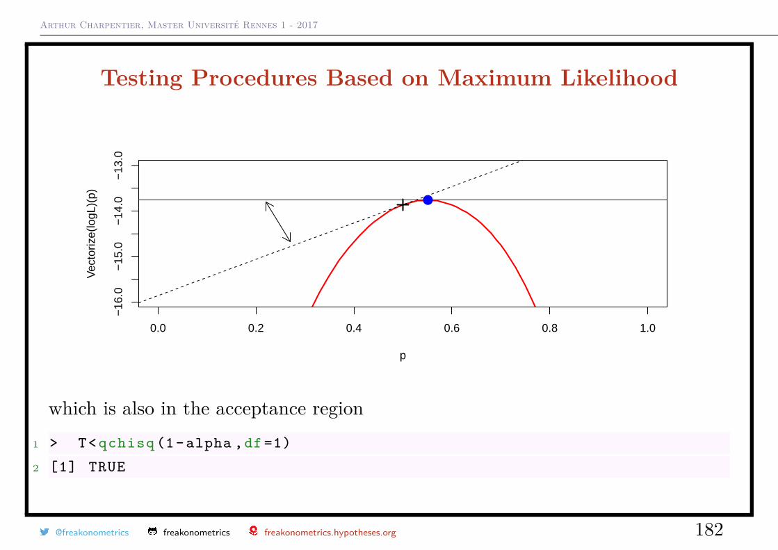
Arthur Charpentier, Master Université Rennes 1 - 2017
Testing Procedures Based on Maximum Likelihood
0.0 0.2 0.4 0.6 0.8 1.0
−16
.0−
15.0
−14
.0−
13.0
p
Vec
toriz
e(lo
gL)(
p)
which is also in the acceptance region1 > T< qchisq (1-alpha ,df =1)
2 [1] TRUE
@freakonometrics freakonometrics freakonometrics.hypotheses.org 182
Arthur Charpentier, Master Université Rennes 1 - 2017
Method of MomentsThe method of moments is probably the most simple and intuitive technique toderive an estimator of θ. If E(X) = g(θ), we should consider θ such that x = g(θ).
For an exponential distribution E(θ), P(X ≤ x) = 1− e−θx, E(X) = 1/θ, andθ = 1/x.
For a uniform distribution on [0, θ], E(X) = θ/2, so θ = 2x.
If θ ∈ R2, we should use two moments, i.e. either Var(X) or E(X2).
@freakonometrics freakonometrics freakonometrics.hypotheses.org 183
Arthur Charpentier, Master Université Rennes 1 - 2017
Comparing EstimatorsStandard propoerties of statistical estimators are
• unbiasedness, E(θn) = θ,• convergence, θn
P→ θ, as n→∞• asymptotic normality,
√n(θ − θ) L→ N (0, σ2) as n→∞,
• efficiency• optimality
Let θ1 and θ2 denote two unbiased estimators, θ1 is said to be more efficient thanθ2 if its variance is smaller.
@freakonometrics freakonometrics freakonometrics.hypotheses.org 184
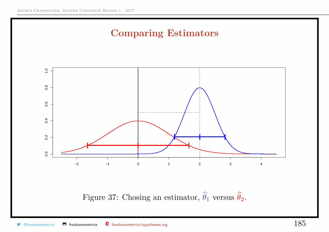
Arthur Charpentier, Master Université Rennes 1 - 2017
Comparing Estimators
−2 −1 0 1 2 3 4
0.0
0.2
0.4
0.6
0.8
1.0
Figure 37: Chosing an estimator, θ1 versus θ2.
@freakonometrics freakonometrics freakonometrics.hypotheses.org 185
Arthur Charpentier, Master Université Rennes 1 - 2017
Comparing Estimators
• θ1 is a biased estimator of θ (E(θ1) 6= E(θ)),
• θ2 is an unbiased estimator of θ (E(θ2) = E(θ)),
• Var(θ1) ≤ Var(θ2).
Estimator θ1 can be interesting if it bias can be estimated, but usually
• bias is a function of θ (which is unkown),
• bias is a complicated function of θ.
@freakonometrics freakonometrics freakonometrics.hypotheses.org 186
Arthur Charpentier, Master Université Rennes 1 - 2017
A short introduction to non-parametric statisticsFor x ∈ R, the cdf is defined as F (x) = P[X ≤ x], so, given a samplex1, x2, · · · , xn, a natural estimator for F (x) is
F (x) = 1n
n∑i=1
1(xi ≤ x),
called the empirical cumulative distribution function.
Consider now a probabilist sample, X1, X2, · · · , Xn, so that
F (x) = 1n
n∑i=1
1(Xi ≤ x)︸ ︷︷ ︸Yi
,
is now a random variable. Yi’s are i.i.d. random variables, with a Bernoullidistribution, Yi ∼ B(p), with p = F (x).
@freakonometrics freakonometrics freakonometrics.hypotheses.org 187
Arthur Charpentier, Master Université Rennes 1 - 2017
A short introduction to non-parametric statisticsThus, nF (x) ∼ B(n, F (x)), and therefore
E[F (x)] = F (x) and Var(F (x)) = F (x) · [1− F (x)]n
.
By the strong law of large numbers, the estimator Fn(t) converges towards F (t)almost surely, for every t
Fn(t) a.s.−−→ F (t)
thus the estimator Fn(t) is consistent.
This is a pointwise convergence of the empirical distribution function
There is a stronger result, called the Glivenko-Cantelli theorem, which statesthat the convergence in fact happens uniformly over t
‖Fn − F‖∞ ≡ supt∈R
∣∣Fn(t)− F (t)∣∣ a.s.−−→ 0.
@freakonometrics freakonometrics freakonometrics.hypotheses.org 188
Arthur Charpentier, Master Université Rennes 1 - 2017
A short introduction to non-parametric statisticsThe left part is called the Kolmogorov-Smirnov statistic, used for testing thegoodness-of-fit between the empirical distribution Fn and the assumed truecumulative distribution function F .
One can also prove that
√n(Fn(t)− F (t)
) d−→ N(
0, F (t)(1− F (t)
)).
(which can be used to get a pointwise confidence interval).
@freakonometrics freakonometrics freakonometrics.hypotheses.org 189
Arthur Charpentier, Master Université Rennes 1 - 2017
A short introduction to non-parametric statisticsWe’ve seen how to estimate (non-parametrically) F . What about the density?
Its kernel density estimator is
fh(x) = 1n
n∑i=1
Kh(x− xi) = 1nh
n∑i=1
K(x− xi
h
),
where K is the kernel — a non-negative function that integrates to one
h > 0 is a smoothing parameter called the bandwidth
A rule-of-thumb bandwidth estimator h =(
4σ5
3n
) 15
≈ 1.06σn−1/5,
@freakonometrics freakonometrics freakonometrics.hypotheses.org 190
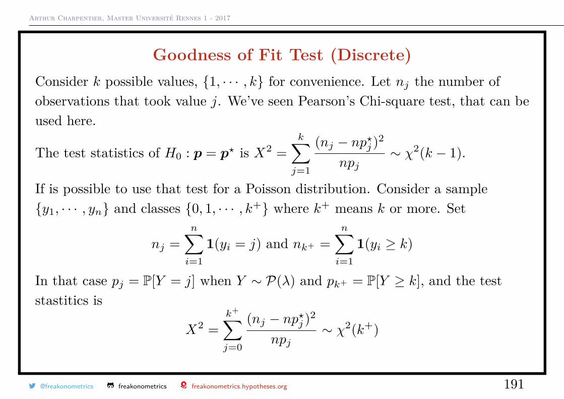
Arthur Charpentier, Master Université Rennes 1 - 2017
Goodness of Fit Test (Discrete)Consider k possible values, 1, · · · , k for convenience. Let nj the number ofobservations that took value j. We’ve seen Pearson’s Chi-square test, that can beused here.
The test statistics of H0 : p = p? is X2 =k∑j=1
(nj − np?j )2
npj∼ χ2(k − 1).
If is possible to use that test for a Poisson distribution. Consider a sampley1, · · · , yn and classes 0, 1, · · · , k+ where k+ means k or more. Set
nj =n∑i=1
1(yi = j) and nk+ =n∑i=1
1(yi ≥ k)
In that case pj = P[Y = j] when Y ∼ P(λ) and pk+ = P[Y ≥ k], and the teststastitics is
X2 =k+∑j=0
(nj − np?j )2
npj∼ χ2(k+)
@freakonometrics freakonometrics freakonometrics.hypotheses.org 191
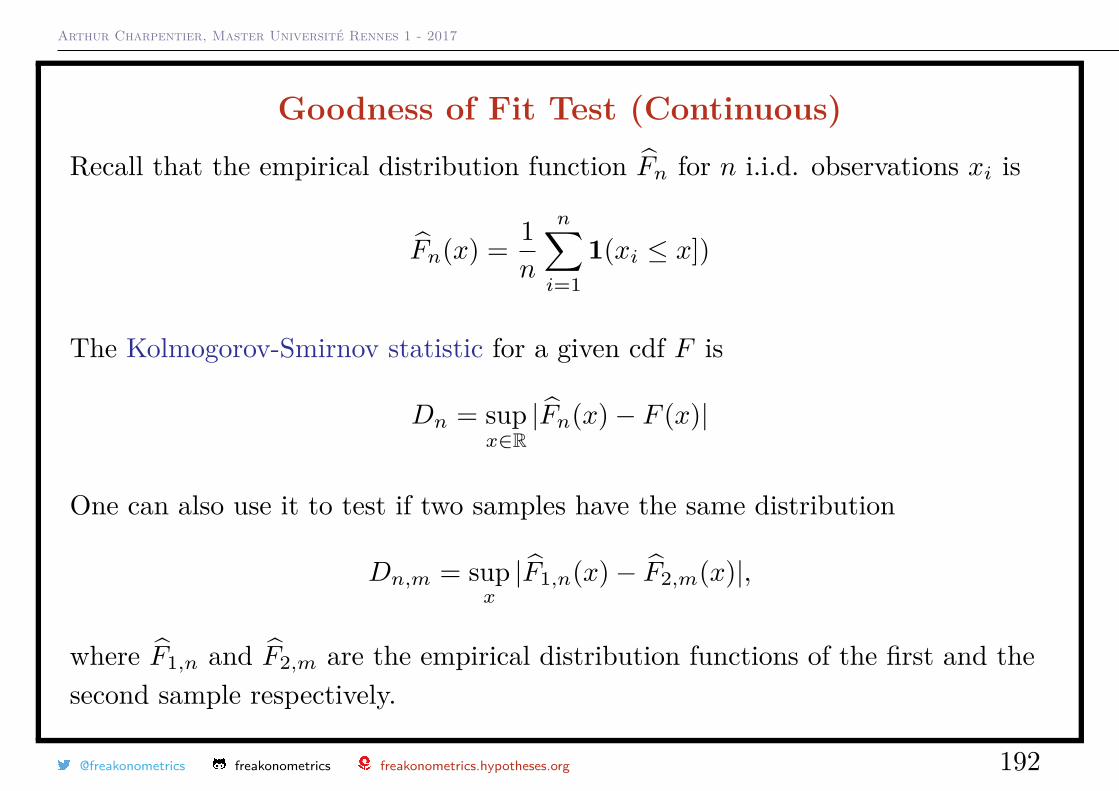
Arthur Charpentier, Master Université Rennes 1 - 2017
Goodness of Fit Test (Continuous)Recall that the empirical distribution function Fn for n i.i.d. observations xi is
Fn(x) = 1n
n∑i=1
1(xi ≤ x])
The Kolmogorov-Smirnov statistic for a given cdf F is
Dn = supx∈R|Fn(x)− F (x)|
One can also use it to test if two samples have the same distribution
Dn,m = supx|F1,n(x)− F2,m(x)|,
where F1,n and F2,m are the empirical distribution functions of the first and thesecond sample respectively.
@freakonometrics freakonometrics freakonometrics.hypotheses.org 192
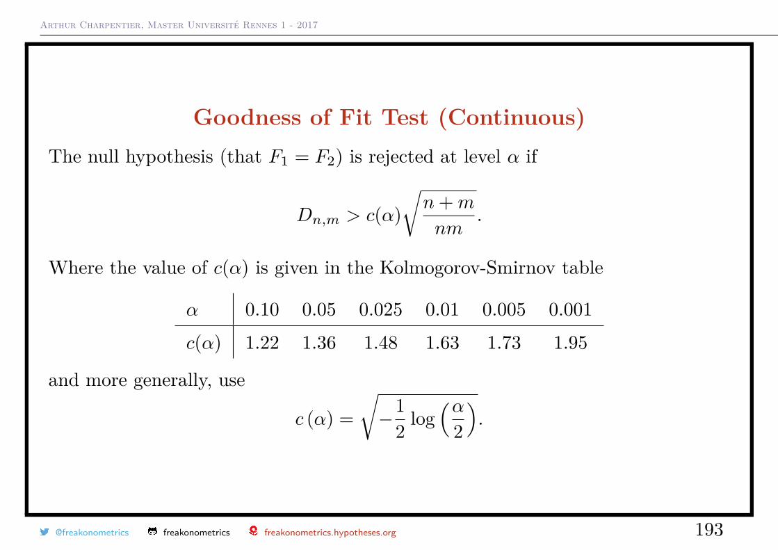
Arthur Charpentier, Master Université Rennes 1 - 2017
Goodness of Fit Test (Continuous)The null hypothesis (that F1 = F2) is rejected at level α if
Dn,m > c(α)√n+m
nm.
Where the value of c(α) is given in the Kolmogorov-Smirnov table
α 0.10 0.05 0.025 0.01 0.005 0.001
c(α) 1.22 1.36 1.48 1.63 1.73 1.95
and more generally, use
c (α) =√−1
2 log(α
2
).
@freakonometrics freakonometrics freakonometrics.hypotheses.org 193